R - 快速指南
R - Overview
R是用于统计分析,图形表示和报告的编程语言和软件环境。 R由新西兰奥克兰大学的Ross Ihaka和Robert Gentleman创建,目前由R Development Core Team开发。
R的核心是解释型计算机语言,它允许分支和循环以及使用函数的模块化编程。 R允许与用C,C ++,。Net,Python或FORTRAN语言编写的过程集成以提高效率。
R在GNU通用公共许可证下免费提供,并且为Linux,Windows和Mac等各种操作系统提供了预编译的二进制版本。
R是在GNU样式副本下分发的自由软件,是GNU项目的官方部分,名为GNU S
R的演变
R最初由Ross Ihaka和Robert Gentleman在新西兰奥克兰的奥克兰大学统计系撰写。 R于1993年首次亮相。
一大群人通过发送代码和错误报告为R做出了贡献。
自1997年中期以来,已有一个核心小组(“R核心小组”)可以修改R源代码档案。
R的特点
如前所述,R是用于统计分析,图形表示和报告的编程语言和软件环境。 以下是R的重要特征 -
R是一种发展良好,简单有效的编程语言,包括条件,循环,用户定义的递归函数以及输入和输出设施。
R拥有有效的数据处理和存储设施,
R为数组,列表,向量和矩阵的计算提供了一套运算符。
R为数据分析提供了大量,连贯和集成的工具集合。
R提供用于数据分析的图形设施,可直接在计算机上显示或在纸张上打印。
作为结论,R是世界上使用最广泛的统计编程语言。 它是数据科学家的首选,并得到了充满活力和才华的贡献者社区的支持。 R在大学教授并部署在关键业务应用程序中。 本教程将通过简单易用的步骤教您R编程以及合适的示例。
R - Environment Setup
本地环境设置 (Local Environment Setup)
如果您仍然愿意为R设置环境,则可以按照以下步骤操作。
Windows安装 (Windows Installation)
您可以从R-3.2.2 for Windows(32/64位)下载R的Windows安装程序版本,并将其保存在本地目录中。
因为它是一个名为“R-version-win.exe”的Windows安装程序(.exe)。 您只需双击并运行安装程序即可接受默认设置。 如果您的Windows是32位版本,则会安装32位版本。 但如果您的Windows是64位,那么它会安装32位和64位版本。
安装后,您可以找到该图标,以便在Windows程序文件下的目录结构“R\R3.2.2\bin\i386\Rgui.exe”中运行本程序。 单击此图标将显示R-GUI,它是进行R编程的R控制台。
Linux安装
R可用作R Binaries位置的许多Linux版本的二进制文件 。
安装Linux的说明因风味而异。 在上述链接中的每种类型的Linux版本中都提到了这些步骤。 但是,如果你赶时间,那么可以使用yum命令安装R,如下所示 -
$ yum install R
上面的命令将安装R编程的核心功能以及标准软件包,还需要额外的软件包,然后你可以按如下方式启动R提示 -
$ R
R version 3.2.0 (2015-04-16) -- "Full of  Ingredients"
Copyright (C) 2015 The R Foundation for Statistical Computing
Platform: x86_64-redhat-linux-gnu (64-bit)
R is free software and comes with ABSOLUTELY NO WARRANTY.
You are welcome to redistribute it under certain conditions.
Type 'license()' or 'licence()' for distribution details.
R is a collaborative project with many  contributors.
Type 'contributors()' for more information and
'citation()' on how to cite R or R packages in publications.
Type 'demo()' for some demos, 'help()' for on-line help, or
'help.start()' for an HTML browser interface to help.
Type 'q()' to quit R.
>
现在,您可以在R提示符下使用install命令来安装所需的包。 例如,以下命令将安装3D图表所需的plotrix包。
> install.packages("plotrix")
R - Basic Syntax
作为惯例,我们将通过编写“Hello,World!”来开始学习R编程。 程序。 根据需要,您可以在R命令提示符下编程,也可以使用R脚本文件编写程序。 让我们逐一检查。
R Command Prompt
一旦设置了R环境,只需在命令提示符下键入以下命令,即可轻松启动R命令提示符 -
$ R
这将启动R解释器,您将得到一个提示>您可以在哪里开始键入您的程序,如下所示 -
> myString <- "Hello, World!"
> print ( myString)
[1] "Hello, World!"
这里第一个语句定义了一个字符串变量myString,我们在其中分配一个字符串“Hello,World!” 然后使用next语句print()来打印存储在变量myString中的值。
R脚本文件
通常,您将通过在脚本文件中编写程序来执行编程,然后在命令提示符下使用名为Rscript的R解释器执行这些脚本。 因此,让我们开始在名为test.R的文本文件中编写以下代码,如下所示 -
# My first program in R Programming
myString <- "Hello, World!"
print ( myString)
将上述代码保存在文件test.R中,并在Linux命令提示符下执行,如下所示。 即使您使用的是Windows或其他系统,语法也将保持不变。
$ Rscript test.R
当我们运行上述程序时,它会产生以下结果。
[1] "Hello, World!"
注释 (Comments)
注释就像帮助R程序中的文本一样,在执行实际程序时,解释器会忽略它们。 在语句开头使用#编写单个注释,如下所示 -
# My first program in R Programming
R不支持多行注释,但你可以执行一个技巧,如下所示 -
if(FALSE) {
   "This is a demo for multi-line comments and it should be put inside either a
      single OR double quote"
}
myString <- "Hello, World!"
print ( myString)
[1] "Hello, World!"
虽然以上评论将由R口译员执行,但它们不会干扰您的实际计划。 你应该把这些评论放在里面,单引号或双引号。
R - Data Types
通常,在使用任何编程语言进行编程时,您需要使用各种变量来存储各种信息。 变量只是用于存储值的保留内存位置。 这意味着,当您创建变量时,您在内存中保留了一些空间。
您可能希望存储各种数据类型的信息,如字符,宽字符,整数,浮点,双浮点,布尔等。根据变量的数据类型,操作系统分配内存并决定可以存储的内容。保留的记忆。
与R中的其他编程语言(如C和Java)相比,变量未声明为某种数据类型。 变量分配有R-Objects,R对象的数据类型成为变量的数据类型。 有许多类型的R对象。 经常使用的是 -
- Vectors
- Lists
- Matrices
- Arrays
- Factors
- 数据框架
这些对象中最简单的是vector object ,这些原子矢量有六种数据类型,也称为六类矢量。 其他R-Objects建立在原子向量之上。
| 数据类型 | 例 | 校验 |
|---|---|---|
| Logical | TRUE, FALSE | 它产生以下结果 - |
| Numeric | 12.3, 5, 999 | 它产生以下结果 - |
| Integer | 2L, 34L, 0L | 它产生以下结果 - |
| Complex | 3 + 2i | 它产生以下结果 - |
| Character | 'a',''good“,”TRUE“,'23 .4' | 它产生以下结果 - |
| Raw | “Hello”存储为48 65 6c 6c 6f | 它产生以下结果 - |
在R编程中,最基本的数据类型是称为vectors的R对象,它们包含不同类的元素,如上所示。 请注意在R中,课程数量不仅限于上述六种类型。 例如,我们可以使用许多原子向量并创建一个其类将成为数组的数组。
Vectors
如果要创建具有多个元素的向量,则应使用c()函数,这意味着将元素组合到向量中。
# Create a vector.
apple <- c('red','green',"yellow")
print(apple)
# Get the class of the vector.
print(class(apple))
当我们执行上面的代码时,它会产生以下结果 -
[1] "red"    "green"  "yellow"
[1] "character"
Lists
列表是一个R对象,它可以在其中包含许多不同类型的元素,如向量,函数甚至其中的另一个列表。
# Create a list.
list1 <- list(c(2,5,3),21.3,sin)
# Print the list.
print(list1)
当我们执行上面的代码时,它会产生以下结果 -
[[1]]
[1] 2 5 3
[[2]]
[1] 21.3
[[3]]
function (x)  .Primitive("sin")
Matrices
矩阵是二维矩形数据集。 可以使用矩阵函数的向量输入创建它。
# Create a matrix.
M = matrix( c('a','a','b','c','b','a'), nrow = 2, ncol = 3, byrow = TRUE)
print(M)
当我们执行上面的代码时,它会产生以下结果 -
     [,1] [,2] [,3]
[1,] "a"  "a"  "b"
[2,] "c"  "b"  "a"
Arrays
虽然矩阵局限于两个维度,但阵列可以具有任意数量的维度。 数组函数采用dim属性创建所需的维度数。 在下面的例子中,我们创建了一个包含两个元素的数组,每个元素都是3x3矩阵。
# Create an array.
a <- array(c('green','yellow'),dim = c(3,3,2))
print(a)
当我们执行上面的代码时,它会产生以下结果 -
, , 1
     [,1]     [,2]     [,3]
[1,] "green"  "yellow" "green"
[2,] "yellow" "green"  "yellow"
[3,] "green"  "yellow" "green"
, , 2
     [,1]     [,2]     [,3]
[1,] "yellow" "green"  "yellow"
[2,] "green"  "yellow" "green"
[3,] "yellow" "green"  "yellow"
Factors
因素是使用向量创建的r对象。 它将向量与向量中元素的不同值一起存储为标签。 无论输入向量中的标签是数字,字符还是布尔等,标签始终都是字符。 它们在统计建模中很有用。
使用factor()函数创建factor() 。 nlevels函数给出了级别的计数。
# Create a vector.
apple_colors <- c('green','green','yellow','red','red','red','green')
# Create a factor object.
factor_apple <- factor(apple_colors)
# Print the factor.
print(factor_apple)
print(nlevels(factor_apple))
当我们执行上面的代码时,它会产生以下结果 -
[1] green  green  yellow red    red    red    green
Levels: green red yellow
[1] 3
数据框架
数据框是表格数据对象。 与数据帧中的矩阵不同,每列可以包含不同的数据模式。 第一列可以是数字,而第二列可以是字符,第三列可以是逻辑列。 它是等长的向量列表。
使用data.frame()函数创建数据框。
# Create the data frame.
BMI <- 	data.frame(
   gender = c("Male", "Male","Female"),
   height = c(152, 171.5, 165),
   weight = c(81,93, 78),
   Age = c(42,38,26)
)
print(BMI)
当我们执行上面的代码时,它会产生以下结果 -
  gender height weight Age
1   Male  152.0     81  42
2   Male  171.5     93  38
3 Female  165.0     78  26
R - Variables
变量为我们提供了程序可以操作的命名存储。 R中的变量可以存储原子矢量,原子矢量组或许多Robjects的组合。 有效的变量名称由字母,数字和点或下划线字符组成。 变量名称以字母或点开头,后面没有数字。
| 变量名 | 合法性 | 原因 |
|---|---|---|
| var_name2. | valid | 有字母,数字,点和下划线 |
| var_name% | Invalid | 字符'%'。 只允许使用点(。)和下划线。 |
| 2var_name | invalid | Starts with a number |
.var_name, var.name | valid | 可以以点(。)开头,但点(。)不应该跟一个数字。 |
| .2var_name | invalid | 起始点后跟一个数字,使其无效。 |
| _var_name | invalid | 以_开头,无效 |
变量分配
可以使用向左,向右和等于运算符为变量赋值。 可以使用print()或cat()函数print()变量的值。 cat()函数将多个项目组合成连续的打印输出。
# Assignment using equal operator.
var.1 = c(0,1,2,3)
# Assignment using leftward operator.
var.2 <- c("learn","R")
# Assignment using rightward operator.
c(TRUE,1) -> var.3
print(var.1)
cat ("var.1 is ", var.1 ,"\n")
cat ("var.2 is ", var.2 ,"\n")
cat ("var.3 is ", var.3 ,"\n")
当我们执行上面的代码时,它会产生以下结果 -
[1] 0 1 2 3
var.1 is  0 1 2 3
var.2 is  learn R
var.3 is  1 1
Note - 向量c(TRUE,1)混合了逻辑和数字类。 因此逻辑类被强制为数字类,使得TRUE为1。
变量的数据类型
在R中,变量本身未声明任何数据类型,而是获取分配给它的R - 对象的数据类型。 所以R被称为动态类型语言,这意味着我们可以在程序中使用它时一次又一次地更改同一变量的变量数据类型。
var_x <- "Hello"
cat("The class of var_x is ",class(var_x),"\n")
var_x <- 34.5
cat("  Now the class of var_x is ",class(var_x),"\n")
var_x <- 27L
cat("   Next the class of var_x becomes ",class(var_x),"\n")
当我们执行上面的代码时,它会产生以下结果 -
The class of var_x is  character
   Now the class of var_x is  numeric
      Next the class of var_x becomes  integer
寻找变量
要了解工作空间中当前可用的所有变量,我们使用ls()函数。 此外,ls()函数可以使用模式来匹配变量名称。
print(ls())
当我们执行上面的代码时,它会产生以下结果 -
[1] "my var"     "my_new_var" "my_var"     "var.1"
[5] "var.2"      "var.3"      "var.name"   "var_name2."
[9] "var_x"      "varname"
Note - 它是一个示例输出,具体取决于环境中声明的变量。
ls()函数可以使用模式匹配变量名称。
# List the variables starting with the pattern "var".
print(ls(pattern = "var"))
当我们执行上面的代码时,它会产生以下结果 -
[1] "my var"     "my_new_var" "my_var"     "var.1"
[5] "var.2"      "var.3"      "var.name"   "var_name2."
[9] "var_x"      "varname"
以dot(.)开头的变量是隐藏的,可以使用ls()函数的“all.names = TRUE”参数列出它们。
print(ls(all.name = TRUE))
当我们执行上面的代码时,它会产生以下结果 -
[1] ".cars"        ".Random.seed" ".var_name"    ".varname"     ".varname2"
[6] "my var"       "my_new_var"   "my_var"       "var.1"        "var.2"
[11]"var.3"        "var.name"     "var_name2."   "var_x"
删除变量
可以使用rm()函数删除变量。 下面我们删除变量var.3。 在打印时,抛出变量错误的值。
rm(var.3)
print(var.3)
当我们执行上面的代码时,它会产生以下结果 -
[1] "var.3"
Error in print(var.3) : object 'var.3' not found
通过一起使用rm()和ls()函数可以删除所有变量。
rm(list = ls())
print(ls())
当我们执行上面的代码时,它会产生以下结果 -
character(0)
R - Operators
运算符是一个符号,告诉编译器执行特定的数学或逻辑操作。 R语言内置运算符丰富,并提供以下类型的运算符。
运算符的类型
我们在R编程中有以下类型的运算符 -
- 算术运算符
- 关系运算符
- 逻辑运算符
- 分配运算符
- 其它运算符
算术运算符 (Arithmetic Operators)
下表显示了R语言支持的算术运算符。 运算符作用于向量的每个元素。
| 操作者 | 描述 | 例 |
|---|---|---|
| + | Adds two vectors | 它产生以下结果 - |
| − | 从第一个中减去第二个向量 | 它产生以下结果 - |
| * | 将两个向量相乘 | 它产生以下结果 - |
| / | 将第一个向量除以第二个向量 | 当我们执行上面的代码时,它会产生以下结果 - |
| %% | 用第二个给出第一个向量的余数 | 它产生以下结果 - |
| %/% | 第一个向量与第二个(商)划分的结果 | 它产生以下结果 - |
| ^ | 第一个向量上升到第二个向量的指数 | 它产生以下结果 - |
关系运算符 (Relational Operators)
下表显示了R语言支持的关系运算符。 将第一矢量的每个元素与第二矢量的相应元素进行比较。 比较结果是布尔值。
| 操作者 | 描述 | 例 |
|---|---|---|
| > | 检查第一个向量的每个元素是否大于第二个向量的对应元素。 | 它产生以下结果 - |
| < | 检查第一个向量的每个元素是否小于第二个向量的对应元素。 | 它产生以下结果 - |
| == | 检查第一个向量的每个元素是否等于第二个向量的对应元素。 | 它产生以下结果 - |
| <= | 检查第一个向量的每个元素是否小于或等于第二个向量的对应元素。 | 它产生以下结果 - |
| >= | 检查第一个向量的每个元素是否大于或等于第二个向量的对应元素。 | 它产生以下结果 - |
| != | 检查第一个向量的每个元素是否与第二个向量的对应元素不相等。 | 它产生以下结果 - |
逻辑运算符 (Logical Operators)
下表显示了R语言支持的逻辑运算符。 它仅适用于逻辑,数字或复杂类型的向量。 所有大于1的数字都被视为逻辑值TRUE。
将第一矢量的每个元素与第二矢量的相应元素进行比较。 比较结果是布尔值。
| 操作者 | 描述 | 例 |
|---|---|---|
| & | 它被称为元素逻辑AND运算符。 它将第一个向量的每个元素与第二个向量的对应元素组合在一起,如果两个元素都为TRUE,则输出TRUE。 | 它产生以下结果 - |
| | | 它被称为元素逻辑OR运算符。 它将第一个向量的每个元素与第二个向量的对应元素组合在一起,如果一个元素为TRUE,则给出输出TRUE。 | 它产生以下结果 - |
| ! | 它被称为Logical NOT运算符。 获取向量的每个元素并给出相反的逻辑值。 | 它产生以下结果 - |
逻辑运算符&&和|| 仅考虑向量的第一个元素,并给出单个元素的向量作为输出。
| 操作者 | 描述 | 例 |
|---|---|---|
| && | 称为逻辑AND运算符。 取两个向量的第一个元素,并且仅当两者都为TRUE时才给出TRUE。 | 它产生以下结果 - |
| || | 称为逻辑OR运算符。 取两个向量的第一个元素,如果其中一个为TRUE则给出TRUE。 | 它产生以下结果 - |
赋值操作符 (Assignment Operators)
这些运算符用于为向量赋值。
| 操作者 | 描述 | 例 |
|---|---|---|
< - 要么 = 要么 << - | Called Left Assignment | 它产生以下结果 - |
- > 要么 - >> | Called Right Assignment | 它产生以下结果 - |
混合操作符 (Miscellaneous Operators)
这些运算符用于特定目的,而不是一般的数学或逻辑计算。
| 操作者 | 描述 | 例 |
|---|---|---|
| : | 冒号运算符。 它为矢量按顺序创建一系列数字。 | 它产生以下结果 - |
| %in% | 此运算符用于标识元素是否属于向量。 | 它产生以下结果 - |
| %*% | 此运算符用于将矩阵与其转置相乘。 | 它产生以下结果 - |
R - Decision making
决策结构要求程序员指定程序要评估或测试的一个或多个条件,以及在条件被确定为true要执行的语句,以及可选的,如果条件要执行的其他语句被认定是false 。
以下是大多数编程语言中常见决策结构的一般形式 -
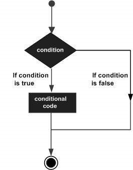
R提供以下类型的决策声明。 单击以下链接以检查其详细信息。
| Sr.No. | 声明和说明 |
|---|---|
| 1 | if 语句 if语句由一个布尔表达式后跟一个或多个语句组成。 |
| 2 | if...else 语句 if语句后面可以跟一个可选的else语句,该语句在布尔表达式为false时执行。 |
| 3 | switch 语句 switch语句允许测试变量与值列表的相等性。 |
R - Loops
可能存在需要多次执行代码块的情况。 通常,语句按顺序执行。 首先执行函数中的第一个语句,然后执行第二个语句,依此类推。
编程语言提供各种控制结构,允许更复杂的执行路径。
循环语句允许我们多次执行语句或语句组,以下是大多数编程语言中循环语句的一般形式 -
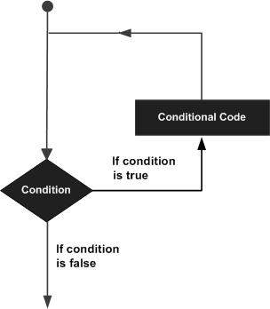
R编程语言提供以下类型的循环来处理循环要求。 单击以下链接以检查其详细信息。
| Sr.No. | 循环类型和描述 |
|---|---|
| 1 | 重复循环 多次执行一系列语句,并缩写管理循环变量的代码。 |
| 2 | 循环 在给定条件为真时重复语句或语句组。 它在执行循环体之前测试条件。 |
| 3 | for循环 像while语句一样,除了它测试循环体末尾的条件。 |
循环控制语句 (Loop Control Statements)
循环控制语句将执行从其正常序列更改。 当执行离开作用域时,将销毁在该作用域中创建的所有自动对象。
R支持以下控制语句。 单击以下链接以检查其详细信息。
| Sr.No. | 控制声明和描述 |
|---|---|
| 1 | break statement 终止loop语句并将执行转移到loop语句。 |
| 2 | Next statement next语句模拟R switch的行为。 |
R - 函数
函数是组合在一起执行特定任务的一组语句。 R具有大量内置函数,用户可以创建自己的函数。
在R中,函数是一个对象,因此R解释器能够将控制传递给函数,以及函数完成操作可能需要的参数。
该函数依次执行其任务并将控制权返回给解释器以及可能存储在其他对象中的任何结果。
函数定义 (Function Definition)
使用关键字function创建R function 。 R函数定义的基本语法如下 -
function_name <- function(arg_1, arg_2, ...) {
   Function body
}
功能组件
功能的不同部分是 -
Function Name - 这是Function Name的实际名称。 它作为具有此名称的对象存储在R环境中。
Arguments - 参数是占位符。 调用函数时,将值传递给参数。 参数是可选的; 也就是说,函数可能不包含任何参数。 参数也可以有默认值。
Function Body - 函数体包含一组语句,用于定义函数的功能。
Return Value - 函数的返回值是要计算的函数体中的最后一个表达式。
R具有许多in-built函数,可以在程序中直接调用而无需先定义它们。 我们还可以创建和使用我们自己的功能,称为user defined功能。
Built-in Function
内置函数的简单示例是seq() , mean() , max() , sum(x)和paste(...)等。它们由用户编写的程序直接调用。 您可以参考最常用的R函数。
# Create a sequence of numbers from 32 to 44.
print(seq(32,44))
# Find mean of numbers from 25 to 82.
print(mean(25:82))
# Find sum of numbers frm 41 to 68.
print(sum(41:68))
当我们执行上面的代码时,它会产生以下结果 -
[1] 32 33 34 35 36 37 38 39 40 41 42 43 44
[1] 53.5
[1] 1526
User-defined Function
我们可以在R中创建用户定义的函数。它们特定于用户想要的内容,一旦创建,就可以像内置函数一样使用它们。 下面是如何创建和使用函数的示例。
# Create a function to print squares of numbers in sequence.
new.function <- function(a) {
   for(i in 1:a) {
      b <- i^2
      print(b)
   }
}
调用一个函数 (Calling a Function)
# Create a function to print squares of numbers in sequence.
new.function <- function(a) {
   for(i in 1:a) {
      b <- i^2
      print(b)
   }
}
# Call the function new.function supplying 6 as an argument.
new.function(6)
当我们执行上面的代码时,它会产生以下结果 -
[1] 1
[1] 4
[1] 9
[1] 16
[1] 25
[1] 36
在没有参数的情况下调用函数
# Create a function without an argument.
new.function <- function() {
   for(i in 1:5) {
      print(i^2)
   }
}
# Call the function without supplying an argument.
new.function()
当我们执行上面的代码时,它会产生以下结果 -
[1] 1
[1] 4
[1] 9
[1] 16
[1] 25
使用参数值调用函数(按位置和名称)
函数调用的参数可以按照函数中定义的相同顺序提供,也可以以不同的顺序提供,但可以分配给参数的名称。
# Create a function with arguments.
new.function <- function(a,b,c) {
   result <- a * b + c
   print(result)
}
# Call the function by position of arguments.
new.function(5,3,11)
# Call the function by names of the arguments.
new.function(a = 11, b = 5, c = 3)
当我们执行上面的代码时,它会产生以下结果 -
[1] 26
[1] 58
使用默认参数调用函数
我们可以在函数定义中定义参数的值,并调用函数而不提供任何参数来获取默认结果。 但我们也可以通过提供参数的新值来调用这些函数,并获得非默认结果。
# Create a function with arguments.
new.function <- function(a = 3, b = 6) {
   result <- a * b
   print(result)
}
# Call the function without giving any argument.
new.function()
# Call the function with giving new values of the argument.
new.function(9,5)
当我们执行上面的代码时,它会产生以下结果 -
[1] 18
[1] 45
懒惰的功能评估
对函数的参数进行了懒惰的计算,这意味着只有在函数体需要时才会对它们进行求值。
# Create a function with arguments.
new.function <- function(a, b) {
   print(a^2)
   print(a)
   print(b)
}
# Evaluate the function without supplying one of the arguments.
new.function(6)
当我们执行上面的代码时,它会产生以下结果 -
[1] 36
[1] 6
Error in print(b) : argument "b" is missing, with no default
R - Strings
在R中的一对单引号或双引号内写入的任何值都被视为字符串。 内部R将每个字符串存储在双引号内,即使您使用单引号创建它们也是如此。
字符串构造中应用的规则
字符串开头和结尾的引号应该是双引号或双引号。 他们不能混在一起。
双引号可以插入到以单引号开头和结尾的字符串中。
单引号可以插入到以双引号开头和结尾的字符串中。
双引号不能插入以双引号开头和结尾的字符串中。
单引号不能插入以单引号开头和结尾的字符串。
有效字符串的示例
以下示例阐明了在R中创建字符串的规则。
a <- 'Start and end with single quote'
print(a)
b <- "Start and end with double quotes"
print(b)
c <- "single quote ' in between double quotes"
print(c)
d <- 'Double quotes " in between single quote'
print(d)
运行上面的代码时,我们得到以下输出 -
[1] "Start and end with single quote"
[1] "Start and end with double quotes"
[1] "single quote ' in between double quote"
[1] "Double quote \" in between single quote"
无效字符串的示例
e <- 'Mixed quotes"
print(e)
f <- 'Single quote ' inside single quote'
print(f)
g <- "Double quotes " inside double quotes"
print(g)
当我们运行脚本时,它无法给出以下结果。
Error: unexpected symbol in:
"print(e)
f <- 'Single"
Execution halted
字符串操作
连接字符串 - paste()函数
R中的许多字符串使用paste()函数进行组合。 它可以将任意数量的参数组合在一起。
语法 (Syntax)
粘贴功能的基本语法是 -
paste(..., sep = " ", collapse = NULL)
以下是所用参数的说明 -
...表示要组合的任意数量的参数。
sep表示参数之间的任何分隔符。 这是可选的。
collapse用于消除两个字符串之间的空间。 但不是一个字符串的两个单词中的空格。
例子 (Example)
a <- "Hello"
b <- 'How'
c <- "are you? "
print(paste(a,b,c))
print(paste(a,b,c, sep = "-"))
print(paste(a,b,c, sep = "", collapse = ""))
当我们执行上面的代码时,它会产生以下结果 -
[1] "Hello How are you? "
[1] "Hello-How-are you? "
[1] "HelloHoware you? "
格式化数字和字符串 - format()函数
可以使用format()函数将数字和字符串格式化为特定样式。
语法 (Syntax)
格式函数的基本语法是 -
format(x, digits, nsmall, scientific, width, justify = c("left", "right", "centre", "none"))
以下是所用参数的说明 -
x是矢量输入。
digits是显示的总位数。
nsmall是小数点右边的最小位数。
scientific设置为TRUE以显示科学记数法。
width表示在开头填充空白时显示的最小宽度。
justify是向左,右或中心显示字符串。
例子 (Example)
# Total number of digits displayed. Last digit rounded off.
result <- format(23.123456789, digits = 9)
print(result)
# Display numbers in scientific notation.
result <- format(c(6, 13.14521), scientific = TRUE)
print(result)
# The minimum number of digits to the right of the decimal point.
result <- format(23.47, nsmall = 5)
print(result)
# Format treats everything as a string.
result <- format(6)
print(result)
# Numbers are padded with blank in the beginning for width.
result <- format(13.7, width = 6)
print(result)
# Left justify strings.
result <- format("Hello", width = 8, justify = "l")
print(result)
# Justfy string with center.
result <- format("Hello", width = 8, justify = "c")
print(result)
当我们执行上面的代码时,它会产生以下结果 -
[1] "23.1234568"
[1] "6.000000e+00" "1.314521e+01"
[1] "23.47000"
[1] "6"
[1] "  13.7"
[1] "Hello   "
[1] " Hello  "
计算字符串中的字符数 - nchar()函数
此函数计算字符串中包含空格的字符数。
语法 (Syntax)
nchar()函数的基本语法是 -
nchar(x)
以下是所用参数的说明 -
x是矢量输入。
例子 (Example)
result <- nchar("Count the number of characters")
print(result)
当我们执行上面的代码时,它会产生以下结果 -
[1] 30
更改大小写 - toupper()和tolower()函数
这些函数改变了字符串字符的大小写。
语法 (Syntax)
toupper()和tolower()函数的基本语法是 -
toupper(x)
tolower(x)
以下是所用参数的说明 -
x是矢量输入。
例子 (Example)
# Changing to Upper case.
result <- toupper("Changing To Upper")
print(result)
# Changing to lower case.
result <- tolower("Changing To Lower")
print(result)
当我们执行上面的代码时,它会产生以下结果 -
[1] "CHANGING TO UPPER"
[1] "changing to lower"
提取字符串的部分 - substring()函数
此函数提取String的部分内容。
语法 (Syntax)
substring()函数的基本语法是 -
substring(x,first,last)
以下是所用参数的说明 -
x是字符向量输入。
first是要提取的第一个字符的位置。
last是要提取的最后一个字符的位置。
例子 (Example)
# Extract characters from 5th to 7th position.
result <- substring("Extract", 5, 7)
print(result)
当我们执行上面的代码时,它会产生以下结果 -
[1] "act"
R - Vectors
向量是最基本的R数据对象,有六种类型的原子向量。 它们是逻辑的,整数的,复数的,复杂的,字符和原始的。
矢量创作
单元素矢量
即使只在R中写入一个值,它也会变成长度为1的向量,并且属于上述向量类型之一。
# Atomic vector of type character.
print("abc");
# Atomic vector of type double.
print(12.5)
# Atomic vector of type integer.
print(63L)
# Atomic vector of type logical.
print(TRUE)
# Atomic vector of type complex.
print(2+3i)
# Atomic vector of type raw.
print(charToRaw('hello'))
当我们执行上面的代码时,它会产生以下结果 -
[1] "abc"
[1] 12.5
[1] 63
[1] TRUE
[1] 2+3i
[1] 68 65 6c 6c 6f
多个元素矢量
Using colon operator with numeric data
# Creating a sequence from 5 to 13.
v <- 5:13
print(v)
# Creating a sequence from 6.6 to 12.6.
v <- 6.6:12.6
print(v)
# If the final element specified does not belong to the sequence then it is discarded.
v <- 3.8:11.4
print(v)
当我们执行上面的代码时,它会产生以下结果 -
[1]  5  6  7  8  9 10 11 12 13
[1]  6.6  7.6  8.6  9.6 10.6 11.6 12.6
[1]  3.8  4.8  5.8  6.8  7.8  8.8  9.8 10.8
Using sequence (Seq.) operator
# Create vector with elements from 5 to 9 incrementing by 0.4.
print(seq(5, 9, by = 0.4))
当我们执行上面的代码时,它会产生以下结果 -
[1] 5.0 5.4 5.8 6.2 6.6 7.0 7.4 7.8 8.2 8.6 9.0
Using the c() function
如果其中一个元素是字符,则非字符值被强制转换为字符类型。
# The logical and numeric values are converted to characters.
s <- c('apple','red',5,TRUE)
print(s)
当我们执行上面的代码时,它会产生以下结果 -
[1] "apple" "red" "5" "TRUE"
访问矢量元素
使用索引访问Vector的元素。 [ ] brackets用于索引。 索引从位置1开始。在索引中赋予负值会从结果中删除该元素。 TRUE , FALSE或0和1也可用于索引。
# Accessing vector elements using position.
t <- c("Sun","Mon","Tue","Wed","Thurs","Fri","Sat")
u <- t[c(2,3,6)]
print(u)
# Accessing vector elements using logical indexing.
v <- t[c(TRUE,FALSE,FALSE,FALSE,FALSE,TRUE,FALSE)]
print(v)
# Accessing vector elements using negative indexing.
x <- t[c(-2,-5)]
print(x)
# Accessing vector elements using 0/1 indexing.
y <- t[c(0,0,0,0,0,0,1)]
print(y)
当我们执行上面的代码时,它会产生以下结果 -
[1] "Mon" "Tue" "Fri"
[1] "Sun" "Fri"
[1] "Sun" "Tue" "Wed" "Fri" "Sat"
[1] "Sun"
矢量操纵
矢量算术
可以添加,减去,相乘或分割两个相同长度的矢量,将结果作为矢量输出。
# Create two vectors.
v1 <- c(3,8,4,5,0,11)
v2 <- c(4,11,0,8,1,2)
# Vector addition.
add.result <- v1+v2
print(add.result)
# Vector subtraction.
sub.result <- v1-v2
print(sub.result)
# Vector multiplication.
multi.result <- v1*v2
print(multi.result)
# Vector division.
divi.result <- v1/v2
print(divi.result)
当我们执行上面的代码时,它会产生以下结果 -
[1]  7 19  4 13  1 13
[1] -1 -3  4 -3 -1  9
[1] 12 88  0 40  0 22
[1] 0.7500000 0.7272727       Inf 0.6250000 0.0000000 5.5000000
矢量元素回收
如果我们将算术运算应用于两个长度不等的向量,那么较短向量的元素将被循环以完成操作。
v1 <- c(3,8,4,5,0,11)
v2 <- c(4,11)
# V2 becomes c(4,11,4,11,4,11)
add.result <- v1+v2
print(add.result)
sub.result <- v1-v2
print(sub.result)
当我们执行上面的代码时,它会产生以下结果 -
[1]  7 19  8 16  4 22
[1] -1 -3  0 -6 -4  0
矢量元素排序
可以使用sort()函数sort()向量中的元素进行排序。
v <- c(3,8,4,5,0,11, -9, 304)
# Sort the elements of the vector.
sort.result <- sort(v)
print(sort.result)
# Sort the elements in the reverse order.
revsort.result <- sort(v, decreasing = TRUE)
print(revsort.result)
# Sorting character vectors.
v <- c("Red","Blue","yellow","violet")
sort.result <- sort(v)
print(sort.result)
# Sorting character vectors in reverse order.
revsort.result <- sort(v, decreasing = TRUE)
print(revsort.result)
当我们执行上面的代码时,它会产生以下结果 -
[1]  -9   0   3   4   5   8  11 304
[1] 304  11   8   5   4   3   0  -9
[1] "Blue"   "Red"    "violet" "yellow"
[1] "yellow" "violet" "Red"    "Blue"
R - Lists
列表是包含不同类型元素的R对象,例如 - 数字,字符串,向量和其中的另一个列表。 列表还可以包含矩阵或函数作为其元素。 List是使用list()函数创建的。
创建列表
以下是创建包含字符串,数字,向量和逻辑值的列表的示例。
# Create a list containing strings, numbers, vectors and a logical
# values.
list_data <- list("Red", "Green", c(21,32,11), TRUE, 51.23, 119.1)
print(list_data)
当我们执行上面的代码时,它会产生以下结果 -
[[1]]
[1] "Red"
[[2]]
[1] "Green"
[[3]]
[1] 21 32 11
[[4]]
[1] TRUE
[[5]]
[1] 51.23
[[6]]
[1] 119.1
命名列表元素
列表元素可以给出名称,可以使用这些名称访问它们。
# Create a list containing a vector, a matrix and a list.
list_data <- list(c("Jan","Feb","Mar"), matrix(c(3,9,5,1,-2,8), nrow = 2),
   list("green",12.3))
# Give names to the elements in the list.
names(list_data) <- c("1st Quarter", "A_Matrix", "A Inner list")
# Show the list.
print(list_data)
当我们执行上面的代码时,它会产生以下结果 -
$`1st_Quarter`
[1] "Jan" "Feb" "Mar"
$A_Matrix
     [,1] [,2] [,3]
[1,]    3    5   -2
[2,]    9    1    8
$A_Inner_list
$A_Inner_list[[1]]
[1] "green"
$A_Inner_list[[2]]
[1] 12.3
访问列表元素
列表的元素可以通过列表中元素的索引访问。 如果是命名列表,也可以使用名称访问它。
我们继续使用上面例子中的列表 -
# Create a list containing a vector, a matrix and a list.
list_data <- list(c("Jan","Feb","Mar"), matrix(c(3,9,5,1,-2,8), nrow = 2),
   list("green",12.3))
# Give names to the elements in the list.
names(list_data) <- c("1st Quarter", "A_Matrix", "A Inner list")
# Access the first element of the list.
print(list_data[1])
# Access the thrid element. As it is also a list, all its elements will be printed.
print(list_data[3])
# Access the list element using the name of the element.
print(list_data$A_Matrix)
当我们执行上面的代码时,它会产生以下结果 -
$`1st_Quarter`
[1] "Jan" "Feb" "Mar"
$A_Inner_list
$A_Inner_list[[1]]
[1] "green"
$A_Inner_list[[2]]
[1] 12.3
     [,1] [,2] [,3]
[1,]    3    5   -2
[2,]    9    1    8
操作列表元素
我们可以添加,删除和更新列表元素,如下所示。 我们只能在列表的末尾添加和删除元素。 但我们可以更新任何元素。
# Create a list containing a vector, a matrix and a list.
list_data <- list(c("Jan","Feb","Mar"), matrix(c(3,9,5,1,-2,8), nrow = 2),
   list("green",12.3))
# Give names to the elements in the list.
names(list_data) <- c("1st Quarter", "A_Matrix", "A Inner list")
# Add element at the end of the list.
list_data[4] <- "New element"
print(list_data[4])
# Remove the last element.
list_data[4] <- NULL
# Print the 4th Element.
print(list_data[4])
# Update the 3rd Element.
list_data[3] <- "updated element"
print(list_data[3])
当我们执行上面的代码时,它会产生以下结果 -
[[1]]
[1] "New element"
$<NA>
NULL
$`A Inner list`
[1] "updated element"
合并列表
通过将所有列表放在一个list()函数中,可以将多个列表合并到一个列表中。
# Create two lists.
list1 <- list(1,2,3)
list2 <- list("Sun","Mon","Tue")
# Merge the two lists.
merged.list <- c(list1,list2)
# Print the merged list.
print(merged.list)
当我们执行上面的代码时,它会产生以下结果 -
[[1]]
[1] 1
[[2]]
[1] 2
[[3]]
[1] 3
[[4]]
[1] "Sun"
[[5]]
[1] "Mon"
[[6]]
[1] "Tue"
将列表转换为矢量
可以将列表转换为向量,以便向量的元素可以用于进一步操作。 在将列表转换为向量之后,可以应用对向量的所有算术运算。 要进行此转换,我们使用unlist()函数。 它将列表作为输入并生成向量。
# Create lists.
list1 <- list(1:5)
print(list1)
list2 <-list(10:14)
print(list2)
# Convert the lists to vectors.
v1 <- unlist(list1)
v2 <- unlist(list2)
print(v1)
print(v2)
# Now add the vectors
result <- v1+v2
print(result)
当我们执行上面的代码时,它会产生以下结果 -
[[1]]
[1] 1 2 3 4 5
[[1]]
[1] 10 11 12 13 14
[1] 1 2 3 4 5
[1] 10 11 12 13 14
[1] 11 13 15 17 19
R - Matrices
矩阵是R对象,其中元素以二维矩形布局排列。 它们包含相同原子类型的元素。 虽然我们可以创建一个只包含字符或只包含逻辑值的矩阵,但它们并没有多大用处。 我们使用包含数字元素的矩阵来用于数学计算。
使用matrix()函数创建Matrix。
语法 (Syntax)
在R中创建矩阵的基本语法是 -
matrix(data, nrow, ncol, byrow, dimnames)
以下是所用参数的说明 -
data是输入向量,它成为矩阵的数据元素。
nrow是要创建的行数。
ncol是要创建的列数。
byrow是一个合乎逻辑的线索。 如果为TRUE,则输入向量元素按行排列。
dimname是分配给行和列的名称。
例子 (Example)
创建一个以数字向量作为输入的矩阵。
# Elements are arranged sequentially by row.
M <- matrix(c(3:14), nrow = 4, byrow = TRUE)
print(M)
# Elements are arranged sequentially by column.
N <- matrix(c(3:14), nrow = 4, byrow = FALSE)
print(N)
# Define the column and row names.
rownames = c("row1", "row2", "row3", "row4")
colnames = c("col1", "col2", "col3")
P <- matrix(c(3:14), nrow = 4, byrow = TRUE, dimnames = list(rownames, colnames))
print(P)
当我们执行上面的代码时,它会产生以下结果 -
     [,1] [,2] [,3]
[1,]    3    4    5
[2,]    6    7    8
[3,]    9   10   11
[4,]   12   13   14
     [,1] [,2] [,3]
[1,]    3    7   11
[2,]    4    8   12
[3,]    5    9   13
[4,]    6   10   14
     col1 col2 col3
row1    3    4    5
row2    6    7    8
row3    9   10   11
row4   12   13   14
访问矩阵的元素
可以使用元素的列和行索引访问矩阵的元素。 我们考虑上面的矩阵P来找到下面的具体元素。
# Define the column and row names.
rownames = c("row1", "row2", "row3", "row4")
colnames = c("col1", "col2", "col3")
# Create the matrix.
P <- matrix(c(3:14), nrow = 4, byrow = TRUE, dimnames = list(rownames, colnames))
# Access the element at 3rd column and 1st row.
print(P[1,3])
# Access the element at 2nd column and 4th row.
print(P[4,2])
# Access only the  2nd row.
print(P[2,])
# Access only the 3rd column.
print(P[,3])
当我们执行上面的代码时,它会产生以下结果 -
[1] 5
[1] 13
col1 col2 col3
   6    7    8
row1 row2 row3 row4
   5    8   11   14
矩阵计算
使用R运算符对矩阵执行各种数学运算。 操作的结果也是一个矩阵。
对于操作中涉及的矩阵,维度(行数和列数)应该相同。
矩阵加法和减法
# Create two 2x3 matrices.
matrix1 <- matrix(c(3, 9, -1, 4, 2, 6), nrow = 2)
print(matrix1)
matrix2 <- matrix(c(5, 2, 0, 9, 3, 4), nrow = 2)
print(matrix2)
# Add the matrices.
result <- matrix1 + matrix2
cat("Result of addition","\n")
print(result)
# Subtract the matrices
result <- matrix1 - matrix2
cat("Result of subtraction","\n")
print(result)
当我们执行上面的代码时,它会产生以下结果 -
     [,1] [,2] [,3]
[1,]    3   -1    2
[2,]    9    4    6
     [,1] [,2] [,3]
[1,]    5    0    3
[2,]    2    9    4
Result of addition
     [,1] [,2] [,3]
[1,]    8   -1    5
[2,]   11   13   10
Result of subtraction
     [,1] [,2] [,3]
[1,]   -2   -1   -1
[2,]    7   -5    2
矩阵乘法和除法
# Create two 2x3 matrices.
matrix1 <- matrix(c(3, 9, -1, 4, 2, 6), nrow = 2)
print(matrix1)
matrix2 <- matrix(c(5, 2, 0, 9, 3, 4), nrow = 2)
print(matrix2)
# Multiply the matrices.
result <- matrix1 * matrix2
cat("Result of multiplication","\n")
print(result)
# Divide the matrices
result <- matrix1/matrix2
cat("Result of division","\n")
print(result)
当我们执行上面的代码时,它会产生以下结果 -
     [,1] [,2] [,3]
[1,]    3   -1    2
[2,]    9    4    6
     [,1] [,2] [,3]
[1,]    5    0    3
[2,]    2    9    4
Result of multiplication
     [,1] [,2] [,3]
[1,]   15    0    6
[2,]   18   36   24
Result of division
     [,1]      [,2]      [,3]
[1,]  0.6      -Inf 0.6666667
[2,]  4.5 0.4444444 1.5000000
R - Arrays
数组是R数据对象,可以存储两个以上的数据。 例如 - 如果我们创建一个维度(2,3,4)数组,那么它会创建4个矩形矩阵,每个矩阵有2行3列。 数组只能存储数据类型。
使用array()函数创建array() 。 它将矢量作为输入,并使用dim参数中的值来创建数组。
例子 (Example)
以下示例创建一个包含两个3x3矩阵的数组,每个矩阵包含3行和3列。
# Create two vectors of different lengths.
vector1 <- c(5,9,3)
vector2 <- c(10,11,12,13,14,15)
# Take these vectors as input to the array.
result <- array(c(vector1,vector2),dim = c(3,3,2))
print(result)
当我们执行上面的代码时,它会产生以下结果 -
, , 1
     [,1] [,2] [,3]
[1,]    5   10   13
[2,]    9   11   14
[3,]    3   12   15
, , 2
     [,1] [,2] [,3]
[1,]    5   10   13
[2,]    9   11   14
[3,]    3   12   15
命名列和行
我们可以使用dimnames参数为数组中的行,列和矩阵dimnames 。
# Create two vectors of different lengths.
vector1 <- c(5,9,3)
vector2 <- c(10,11,12,13,14,15)
column.names <- c("COL1","COL2","COL3")
row.names <- c("ROW1","ROW2","ROW3")
matrix.names <- c("Matrix1","Matrix2")
# Take these vectors as input to the array.
result <- array(c(vector1,vector2),dim = c(3,3,2),dimnames = list(row.names,column.names,
   matrix.names))
print(result)
当我们执行上面的代码时,它会产生以下结果 -
, , Matrix1
     COL1 COL2 COL3
ROW1    5   10   13
ROW2    9   11   14
ROW3    3   12   15
, , Matrix2
     COL1 COL2 COL3
ROW1    5   10   13
ROW2    9   11   14
ROW3    3   12   15
访问数组元素 (Accessing Array Elements)
# Create two vectors of different lengths.
vector1 <- c(5,9,3)
vector2 <- c(10,11,12,13,14,15)
column.names <- c("COL1","COL2","COL3")
row.names <- c("ROW1","ROW2","ROW3")
matrix.names <- c("Matrix1","Matrix2")
# Take these vectors as input to the array.
result <- array(c(vector1,vector2),dim = c(3,3,2),dimnames = list(row.names,
   column.names, matrix.names))
# Print the third row of the second matrix of the array.
print(result[3,,2])
# Print the element in the 1st row and 3rd column of the 1st matrix.
print(result[1,3,1])
# Print the 2nd Matrix.
print(result[,,2])
当我们执行上面的代码时,它会产生以下结果 -
COL1 COL2 COL3
   3   12   15
[1] 13
     COL1 COL2 COL3
ROW1    5   10   13
ROW2    9   11   14
ROW3    3   12   15
操纵数组元素
由于数组由多维构成矩阵,因此通过访问矩阵的元素来执行对数组元素的操作。
# Create two vectors of different lengths.
vector1 <- c(5,9,3)
vector2 <- c(10,11,12,13,14,15)
# Take these vectors as input to the array.
array1 <- array(c(vector1,vector2),dim = c(3,3,2))
# Create two vectors of different lengths.
vector3 <- c(9,1,0)
vector4 <- c(6,0,11,3,14,1,2,6,9)
array2 <- array(c(vector1,vector2),dim = c(3,3,2))
# create matrices from these arrays.
matrix1 <- array1[,,2]
matrix2 <- array2[,,2]
# Add the matrices.
result <- matrix1+matrix2
print(result)
当我们执行上面的代码时,它会产生以下结果 -
     [,1] [,2] [,3]
[1,]   10   20   26
[2,]   18   22   28
[3,]    6   24   30
跨数组元素的计算
我们可以使用apply()函数对数组中的元素进行计算。
语法 (Syntax)
apply(x, margin, fun)
以下是所用参数的说明 -
x是一个数组。
margin是使用的数据集的名称。
fun是要跨数组元素应用的函数。
例子 (Example)
我们使用下面的apply()函数计算所有矩阵中数组行中元素的总和。
# Create two vectors of different lengths.
vector1 <- c(5,9,3)
vector2 <- c(10,11,12,13,14,15)
# Take these vectors as input to the array.
new.array <- array(c(vector1,vector2),dim = c(3,3,2))
print(new.array)
# Use apply to calculate the sum of the rows across all the matrices.
result <- apply(new.array, c(1), sum)
print(result)
当我们执行上面的代码时,它会产生以下结果 -
, , 1
     [,1] [,2] [,3]
[1,]    5   10   13
[2,]    9   11   14
[3,]    3   12   15
, , 2
     [,1] [,2] [,3]
[1,]    5   10   13
[2,]    9   11   14
[3,]    3   12   15
[1] 56 68 60
R - Factors
因素是数据对象,用于对数据进行分类并将其存储为级别。 它们可以存储字符串和整数。 它们在具有有限数量的唯一值的列中很有用。 像“男性”,“女性”和“真,假”等。它们在统计建模的数据分析中很有用。
通过将矢量作为输入,使用factor ()函数创建factor () 。
例子 (Example)
# Create a vector as input.
data <- c("East","West","East","North","North","East","West","West","West","East","North")
print(data)
print(is.factor(data))
# Apply the factor function.
factor_data <- factor(data)
print(factor_data)
print(is.factor(factor_data))
当我们执行上面的代码时,它会产生以下结果 -
[1] "East"  "West"  "East"  "North" "North" "East"  "West"  "West"  "West"  "East" "North"
[1] FALSE
[1] East  West  East  North North East  West  West  West  East  North
Levels: East North West
[1] TRUE
数据框架中的因素
在使用一列文本数据创建任何数据框时,R将文本列视为分类数据并在其上创建因子。
# Create the vectors for data frame.
height <- c(132,151,162,139,166,147,122)
weight <- c(48,49,66,53,67,52,40)
gender <- c("male","male","female","female","male","female","male")
# Create the data frame.
input_data <- data.frame(height,weight,gender)
print(input_data)
# Test if the gender column is a factor.
print(is.factor(input_data$gender))
# Print the gender column so see the levels.
print(input_data$gender)
当我们执行上面的代码时,它会产生以下结果 -
  height weight gender
1    132     48   male
2    151     49   male
3    162     66 female
4    139     53 female
5    166     67   male
6    147     52 female
7    122     40   male
[1] TRUE
[1] male   male   female female male   female male
Levels: female male
改变级别顺序
通过使用新的级别顺序再次应用因子函数,可以改变因子中级别的顺序。
data <- c("East","West","East","North","North","East","West",
   "West","West","East","North")
# Create the factors
factor_data <- factor(data)
print(factor_data)
# Apply the factor function with required order of the level.
new_order_data <- factor(factor_data,levels = c("East","West","North"))
print(new_order_data)
当我们执行上面的代码时,它会产生以下结果 -
 [1] East  West  East  North North East  West  West  West  East  North
Levels: East North West
 [1] East  West  East  North North East  West  West  West  East  North
Levels: East West North
生成因子水平
我们可以使用gl()函数生成因子级别。 它需要两个整数作为输入,表示每个级别有多少级别和多少次。
语法 (Syntax)
gl(n, k, labels)
以下是所用参数的说明 -
n是一个给出级别数的整数。
k是给出复制次数的整数。
labels是结果因子水平的标签矢量。
例子 (Example)
v <- gl(3, 4, labels = c("Tampa", "Seattle","Boston"))
print(v)
当我们执行上面的代码时,它会产生以下结果 -
Tampa   Tampa   Tampa   Tampa   Seattle Seattle Seattle Seattle Boston
[10] Boston  Boston  Boston
Levels: Tampa Seattle Boston
R - Data Frames
数据框是一个表或二维数组结构,其中每列包含一个变量的值,每行包含每列的一组值。
以下是数据框的特征。
- 列名称应为非空。
- 行名称应该是唯一的。
- 存储在数据帧中的数据可以是数字,因子或字符类型。
- 每列应包含相同数量的数据项。
创建数据框
# Create the data frame.
emp.data <- data.frame(
   emp_id = c (1:5),
   emp_name = c("Rick","Dan","Michelle","Ryan","Gary"),
   salary = c(623.3,515.2,611.0,729.0,843.25),
   start_date = as.Date(c("2012-01-01", "2013-09-23", "2014-11-15", "2014-05-11",
      "2015-03-27")),
   stringsAsFactors = FALSE
)
# Print the data frame.
print(emp.data)
当我们执行上面的代码时,它会产生以下结果 -
 emp_id    emp_name     salary     start_date
1     1     Rick        623.30     2012-01-01
2     2     Dan         515.20     2013-09-23
3     3     Michelle    611.00     2014-11-15
4     4     Ryan        729.00     2014-05-11
5     5     Gary        843.25     2015-03-27
获取数据框架的结构
通过使用str()函数可以看到数据框的结构。
# Create the data frame.
emp.data <- data.frame(
   emp_id = c (1:5),
   emp_name = c("Rick","Dan","Michelle","Ryan","Gary"),
   salary = c(623.3,515.2,611.0,729.0,843.25),
   start_date = as.Date(c("2012-01-01", "2013-09-23", "2014-11-15", "2014-05-11",
      "2015-03-27")),
   stringsAsFactors = FALSE
)
# Get the structure of the data frame.
str(emp.data)
当我们执行上面的代码时,它会产生以下结果 -
'data.frame':   5 obs. of  4 variables:
 $ emp_id    : int  1 2 3 4 5
 $ emp_name  : chr  "Rick" "Dan" "Michelle" "Ryan" ...
 $ salary    : num  623 515 611 729 843
 $ start_date: Date, format: "2012-01-01" "2013-09-23" "2014-11-15" "2014-05-11" ...
数据框中的数据摘要
可以通过应用summary()函数获得数据的统计摘要和性质。
# Create the data frame.
emp.data <- data.frame(
   emp_id = c (1:5),
   emp_name = c("Rick","Dan","Michelle","Ryan","Gary"),
   salary = c(623.3,515.2,611.0,729.0,843.25),
   start_date = as.Date(c("2012-01-01", "2013-09-23", "2014-11-15", "2014-05-11",
      "2015-03-27")),
   stringsAsFactors = FALSE
)
# Print the summary.
print(summary(emp.data))
当我们执行上面的代码时,它会产生以下结果 -
     emp_id    emp_name             salary        start_date
 Min.   :1   Length:5           Min.   :515.2   Min.   :2012-01-01
 1st Qu.:2   Class :character   1st Qu.:611.0   1st Qu.:2013-09-23
 Median :3   Mode  :character   Median :623.3   Median :2014-05-11
 Mean   :3                      Mean   :664.4   Mean   :2014-01-14
 3rd Qu.:4                      3rd Qu.:729.0   3rd Qu.:2014-11-15
 Max.   :5                      Max.   :843.2   Max.   :2015-03-27
从数据框中提取数据
使用列名从数据框中提取特定列。
# Create the data frame.
emp.data <- data.frame(
   emp_id = c (1:5),
   emp_name = c("Rick","Dan","Michelle","Ryan","Gary"),
   salary = c(623.3,515.2,611.0,729.0,843.25),
   start_date = as.Date(c("2012-01-01","2013-09-23","2014-11-15","2014-05-11",
      "2015-03-27")),
   stringsAsFactors = FALSE
)
# Extract Specific columns.
result <- data.frame(emp.data$emp_name,emp.data$salary)
print(result)
当我们执行上面的代码时,它会产生以下结果 -
  emp.data.emp_name emp.data.salary
1              Rick          623.30
2               Dan          515.20
3          Michelle          611.00
4              Ryan          729.00
5              Gary          843.25
提取前两行,然后提取所有列
# Create the data frame.
emp.data <- data.frame(
   emp_id = c (1:5),
   emp_name = c("Rick","Dan","Michelle","Ryan","Gary"),
   salary = c(623.3,515.2,611.0,729.0,843.25),
   start_date = as.Date(c("2012-01-01", "2013-09-23", "2014-11-15", "2014-05-11",
      "2015-03-27")),
   stringsAsFactors = FALSE
)
# Extract first two rows.
result <- emp.data[1:2,]
print(result)
当我们执行上面的代码时,它会产生以下结果 -
  emp_id    emp_name   salary    start_date
1      1     Rick      623.3     2012-01-01
2      2     Dan       515.2     2013-09-23
用第2和第 4列提取第3行和第 5行
# Create the data frame.
emp.data <- data.frame(
   emp_id = c (1:5),
   emp_name = c("Rick","Dan","Michelle","Ryan","Gary"),
   salary = c(623.3,515.2,611.0,729.0,843.25),
	start_date = as.Date(c("2012-01-01", "2013-09-23", "2014-11-15", "2014-05-11",
      "2015-03-27")),
   stringsAsFactors = FALSE
)
# Extract 3rd and 5th row with 2nd and 4th column.
result <- emp.data[c(3,5),c(2,4)]
print(result)
当我们执行上面的代码时,它会产生以下结果 -
  emp_name start_date
3 Michelle 2014-11-15
5     Gary 2015-03-27
展开数据框
可以通过添加列和行来扩展数据框。
添加列
只需使用新列名添加列向量。
# Create the data frame.
emp.data <- data.frame(
   emp_id = c (1:5),
   emp_name = c("Rick","Dan","Michelle","Ryan","Gary"),
   salary = c(623.3,515.2,611.0,729.0,843.25),
   start_date = as.Date(c("2012-01-01", "2013-09-23", "2014-11-15", "2014-05-11",
      "2015-03-27")),
   stringsAsFactors = FALSE
)
# Add the "dept" coulmn.
emp.data$dept <- c("IT","Operations","IT","HR","Finance")
v <- emp.data
print(v)
当我们执行上面的代码时,它会产生以下结果 -
  emp_id   emp_name    salary    start_date       dept
1     1    Rick        623.30    2012-01-01       IT
2     2    Dan         515.20    2013-09-23       Operations
3     3    Michelle    611.00    2014-11-15       IT
4     4    Ryan        729.00    2014-05-11       HR
5     5    Gary        843.25    2015-03-27       Finance
添加行
要永久地向现有数据框添加更多行,我们需要在与现有数据框相同的结构中引入新行,并使用rbind()函数。
在下面的示例中,我们创建一个包含新行的数据框,并将其与现有数据框合并以创建最终数据框。
# Create the first data frame.
emp.data <- data.frame(
   emp_id = c (1:5),
   emp_name = c("Rick","Dan","Michelle","Ryan","Gary"),
   salary = c(623.3,515.2,611.0,729.0,843.25),
   start_date = as.Date(c("2012-01-01", "2013-09-23", "2014-11-15", "2014-05-11",
      "2015-03-27")),
   dept = c("IT","Operations","IT","HR","Finance"),
   stringsAsFactors = FALSE
)
# Create the second data frame
emp.newdata <- 	data.frame(
   emp_id = c (6:8),
   emp_name = c("Rasmi","Pranab","Tusar"),
   salary = c(578.0,722.5,632.8),
   start_date = as.Date(c("2013-05-21","2013-07-30","2014-06-17")),
   dept = c("IT","Operations","Fianance"),
   stringsAsFactors = FALSE
)
# Bind the two data frames.
emp.finaldata <- rbind(emp.data,emp.newdata)
print(emp.finaldata)
当我们执行上面的代码时,它会产生以下结果 -
  emp_id     emp_name    salary     start_date       dept
1      1     Rick        623.30     2012-01-01       IT
2      2     Dan         515.20     2013-09-23       Operations
3      3     Michelle    611.00     2014-11-15       IT
4      4     Ryan        729.00     2014-05-11       HR
5      5     Gary        843.25     2015-03-27       Finance
6      6     Rasmi       578.00     2013-05-21       IT
7      7     Pranab      722.50     2013-07-30       Operations
8      8     Tusar       632.80     2014-06-17       Fianance
R - Packages
R包是R函数的集合,包含代码和样本数据。 它们存储在R环境中名为"library"的目录下。 默认情况下,R在安装期间安装一组软件包。 当某些特定用途需要时,会在以后添加更多软件包。 当我们启动R控制台时,默认情况下只有默认包可用。 必须明确加载已安装的其他软件包,以供将要使用它们的R程序使用。
所有R语言版本的软件包都列在R软件包中。
以下是用于检查,验证和使用R软件包的命令列表。
检查可用的R包
获取包含R包的库位置
.libPaths()
当我们执行上面的代码时,它会产生以下结果。 它可能会有所不同,具体取决于您的电脑的本地设置。
[2] "C:/Program Files/R/R-3.2.2/library"
获取所有已安装软件包的列表
library()
当我们执行上面的代码时,它会产生以下结果。 它可能会有所不同,具体取决于您的电脑的本地设置。
Packages in library ‘C:/Program Files/R/R-3.2.2/library’:
base                    The R Base Package
boot                    Bootstrap Functions (Originally by Angelo Canty
                        for S)
class                   Functions for Classification
cluster                 "Finding Groups in Data": Cluster Analysis
                        Extended Rousseeuw et al.
codetools               Code Analysis Tools for R
compiler                The R Compiler Package
datasets                The R Datasets Package
foreign                 Read Data Stored by 'Minitab', 'S', 'SAS',
                        'SPSS', 'Stata', 'Systat', 'Weka', 'dBase', ...
graphics                The R Graphics Package
grDevices               The R Graphics Devices and Support for Colours
                        and Fonts
grid                    The Grid Graphics Package
KernSmooth              Functions for Kernel Smoothing Supporting Wand
                        & Jones (1995)
lattice                 Trellis Graphics for R
MASS                    Support Functions and Datasets for Venables and
                        Ripley's MASS
Matrix                  Sparse and Dense Matrix Classes and Methods
methods                 Formal Methods and Classes
mgcv                    Mixed GAM Computation Vehicle with GCV/AIC/REML
                        Smoothness Estimation
nlme                    Linear and Nonlinear Mixed Effects Models
nnet                    Feed-Forward Neural Networks and Multinomial
                        Log-Linear Models
parallel                Support for Parallel computation in R
rpart                   Recursive Partitioning and Regression Trees
spatial                 Functions for Kriging and Point Pattern
                        Analysis
splines                 Regression Spline Functions and Classes
stats                   The R Stats Package
stats4                  Statistical Functions using S4 Classes
survival                Survival Analysis
tcltk                   Tcl/Tk Interface
tools                   Tools for Package Development
utils                   The R Utils Package
获取当前在R环境中加载的所有包
search()
当我们执行上面的代码时,它会产生以下结果。 它可能会有所不同,具体取决于您的电脑的本地设置。
[1] ".GlobalEnv"        "package:stats"     "package:graphics"
[4] "package:grDevices" "package:utils"     "package:datasets"
[7] "package:methods"   "Autoloads"         "package:base"
安装新包
有两种方法可以添加新的R包。 一种是直接从CRAN目录安装,另一种是将软件包下载到本地系统并手动安装。
直接从CRAN安装
以下命令直接从CRAN网页获取软件包,并在R环境中安装软件包。 系统可能会提示您选择最近的镜像。 选择适合您所在位置的那个。
 install.packages("Package Name")
# Install the package named "XML".
 install.packages("XML")
手动安装包
转到链接R Packages以下载所需的包。 将程序包保存为本地系统中适当位置的.zip文件。
现在,您可以运行以下命令在R环境中安装此程序包。
install.packages(file_name_with_path, repos = NULL, type = "source")
# Install the package named "XML"
install.packages("E:/XML_3.98-1.3.zip", repos = NULL, type = "source")
将包加载到库
在可以在代码中使用包之前,必须将其加载到当前的R环境中。 您还需要加载先前已安装但在当前环境中不可用的软件包。
使用以下命令加载包 -
library("package Name", lib.loc = "path to library")
# Load the package named "XML"
install.packages("E:/XML_3.98-1.3.zip", repos = NULL, type = "source")
R - Data Reshaping
R中的数据重塑是关于改变数据组织成行和列的方式。 大多数情况下,R中的数据处理是通过将输入数据作为数据帧来完成的。 从数据帧的行和列中提取数据很容易,但有些情况下我们需要的数据帧格式与我们收到它的格式不同。 R具有许多功能,可以在数据帧中拆分,合并和更改行到列,反之亦然。
在数据框中加入列和行
我们可以使用cbind()函数连接多个向量来创建数据框。 我们也可以使用rbind()函数合并两个数据帧。
# Create vector objects.
city <- c("Tampa","Seattle","Hartford","Denver")
state <- c("FL","WA","CT","CO")
zipcode <- c(33602,98104,06161,80294)
# Combine above three vectors into one data frame.
addresses <- cbind(city,state,zipcode)
# Print a header.
cat("# # # # The First data frame\n")
# Print the data frame.
print(addresses)
# Create another data frame with similar columns
new.address <- data.frame(
   city = c("Lowry","Charlotte"),
   state = c("CO","FL"),
   zipcode = c("80230","33949"),
   stringsAsFactors = FALSE
)
# Print a header.
cat("# # # The Second data frame\n")
# Print the data frame.
print(new.address)
# Combine rows form both the data frames.
all.addresses <- rbind(addresses,new.address)
# Print a header.
cat("# # # The combined data frame\n")
# Print the result.
print(all.addresses)
当我们执行上面的代码时,它会产生以下结果 -
# # # # The First data frame
     city       state zipcode
[1,] "Tampa"    "FL"  "33602"
[2,] "Seattle"  "WA"  "98104"
[3,] "Hartford" "CT"   "6161"
[4,] "Denver"   "CO"  "80294"
# # # The Second data frame
       city       state   zipcode
1      Lowry      CO      80230
2      Charlotte  FL      33949
# # # The combined data frame
       city      state zipcode
1      Tampa     FL    33602
2      Seattle   WA    98104
3      Hartford  CT     6161
4      Denver    CO    80294
5      Lowry     CO    80230
6     Charlotte  FL    33949
合并数据框架
我们可以使用merge()函数合并两个数据帧。 数据框必须具有相同的列名称才能进行合并。
在下面的示例中,我们考虑了Pima Indian Women中的糖尿病数据集,其库名为“MASS”。 我们基于血压(“bp”)和体重指数(“bmi”)的值合并两个数据集。 在选择这两列用于合并时,这两个变量的值在两个数据集中匹配的记录被组合在一起以形成单个数据帧。
library(MASS)
merged.Pima <- merge(x = Pima.te, y = Pima.tr,
   by.x = c("bp", "bmi"),
   by.y = c("bp", "bmi")
)
print(merged.Pima)
nrow(merged.Pima)
当我们执行上面的代码时,它会产生以下结果 -
   bp  bmi npreg.x glu.x skin.x ped.x age.x type.x npreg.y glu.y skin.y ped.y
1  60 33.8       1   117     23 0.466    27     No       2   125     20 0.088
2  64 29.7       2    75     24 0.370    33     No       2   100     23 0.368
3  64 31.2       5   189     33 0.583    29    Yes       3   158     13 0.295
4  64 33.2       4   117     27 0.230    24     No       1    96     27 0.289
5  66 38.1       3   115     39 0.150    28     No       1   114     36 0.289
6  68 38.5       2   100     25 0.324    26     No       7   129     49 0.439
7  70 27.4       1   116     28 0.204    21     No       0   124     20 0.254
8  70 33.1       4    91     32 0.446    22     No       9   123     44 0.374
9  70 35.4       9   124     33 0.282    34     No       6   134     23 0.542
10 72 25.6       1   157     21 0.123    24     No       4    99     17 0.294
11 72 37.7       5    95     33 0.370    27     No       6   103     32 0.324
12 74 25.9       9   134     33 0.460    81     No       8   126     38 0.162
13 74 25.9       1    95     21 0.673    36     No       8   126     38 0.162
14 78 27.6       5    88     30 0.258    37     No       6   125     31 0.565
15 78 27.6      10   122     31 0.512    45     No       6   125     31 0.565
16 78 39.4       2   112     50 0.175    24     No       4   112     40 0.236
17 88 34.5       1   117     24 0.403    40    Yes       4   127     11 0.598
   age.y type.y
1     31     No
2     21     No
3     24     No
4     21     No
5     21     No
6     43    Yes
7     36    Yes
8     40     No
9     29    Yes
10    28     No
11    55     No
12    39     No
13    39     No
14    49    Yes
15    49    Yes
16    38     No
17    28     No
[1] 17
熔化和铸造
R编程最有趣的一个方面是以多个步骤改变数据的形状以获得所需的形状。 用于执行此操作的函数称为melt()和cast() 。
我们认为名为“MASS”的库中存在称为船舶的数据集。
library(MASS)
print(ships)
当我们执行上面的代码时,它会产生以下结果 -
     type year   period   service   incidents
1     A   60     60        127         0
2     A   60     75         63         0
3     A   65     60       1095         3
4     A   65     75       1095         4
5     A   70     60       1512         6
.............
.............
8     A   75     75       2244         11
9     B   60     60      44882         39
10    B   60     75      17176         29
11    B   65     60      28609         58
............
............
17    C   60     60      1179          1
18    C   60     75       552          1
19    C   65     60       781          0
............
............
融化数据
现在我们将数据融合以组织它,将除type和year之外的所有列转换为多行。
molten.ships <- melt(ships, id = c("type","year"))
print(molten.ships)
当我们执行上面的代码时,它会产生以下结果 -
      type year  variable  value
1      A   60    period      60
2      A   60    period      75
3      A   65    period      60
4      A   65    period      75
............
............
9      B   60    period      60
10     B   60    period      75
11     B   65    period      60
12     B   65    period      75
13     B   70    period      60
...........
...........
41     A   60    service    127
42     A   60    service     63
43     A   65    service   1095
...........
...........
70     D   70    service   1208
71     D   75    service      0
72     D   75    service   2051
73     E   60    service     45
74     E   60    service      0
75     E   65    service    789
...........
...........
101    C   70    incidents    6
102    C   70    incidents    2
103    C   75    incidents    0
104    C   75    incidents    1
105    D   60    incidents    0
106    D   60    incidents    0
...........
...........
投下熔融数据
我们可以将熔融数据转换为新形式,其中每年创建每种类型船舶的总量。 它是使用cast()函数完成的。
recasted.ship <- cast(molten.ships, type+year~variable,sum)
print(recasted.ship)
当我们执行上面的代码时,它会产生以下结果 -
     type year  period  service  incidents
1     A   60    135       190      0
2     A   65    135      2190      7
3     A   70    135      4865     24
4     A   75    135      2244     11
5     B   60    135     62058     68
6     B   65    135     48979    111
7     B   70    135     20163     56
8     B   75    135      7117     18
9     C   60    135      1731      2
10    C   65    135      1457      1
11    C   70    135      2731      8
12    C   75    135       274      1
13    D   60    135       356      0
14    D   65    135       480      0
15    D   70    135      1557     13
16    D   75    135      2051      4
17    E   60    135        45      0
18    E   65    135      1226     14
19    E   70    135      3318     17
20    E   75    135       542      1
R - CSV Files
在R中,我们可以从存储在R环境之外的文件中读取数据。 我们还可以将数据写入文件,这些文件将由操作系统存储和访问。 R可以读写各种文件格式,如csv,excel,xml等。
在本章中,我们将学习从csv文件中读取数据,然后将数据写入csv文件。 该文件应存在于当前工作目录中,以便R可以读取它。 当然我们也可以设置自己的目录并从那里读取文件。
获取和设置工作目录
您可以使用getwd()函数检查R工作区指向的目录。 您还可以使用setwd()函数设置新的工作目录。
# Get and print current working directory.
print(getwd())
# Set current working directory.
setwd("/web/com")
# Get and print current working directory.
print(getwd())
当我们执行上面的代码时,它会产生以下结果 -
[1] "/web/com/1441086124_2016"
[1] "/web/com"
此结果取决于您的操作系统和您当前工作的目录。
输入为CSV文件
csv文件是一个文本文件,其中列中的值用逗号分隔。 让我们考虑名为input.csv的文件中存在以下数据。
您可以通过复制和粘贴此数据使用Windows记事本创建此文件。 使用记事本中的“另存为所有文件(*。*)”选项将文件另存为input.csv 。
id,name,salary,start_date,dept
1,Rick,623.3,2012-01-01,IT
2,Dan,515.2,2013-09-23,Operations
3,Michelle,611,2014-11-15,IT
4,Ryan,729,2014-05-11,HR
5,Gary,843.25,2015-03-27,Finance
6,Nina,578,2013-05-21,IT
7,Simon,632.8,2013-07-30,Operations
8,Guru,722.5,2014-06-17,Finance
读取CSV文件
以下是read.csv()函数的一个简单示例,用于读取当前工作目录中可用的CSV文件 -
data <- read.csv("input.csv")
print(data)
当我们执行上面的代码时,它会产生以下结果 -
      id,   name,    salary,   start_date,     dept
1      1    Rick     623.30    2012-01-01      IT
2      2    Dan      515.20    2013-09-23      Operations
3      3    Michelle 611.00    2014-11-15      IT
4      4    Ryan     729.00    2014-05-11      HR
5     NA    Gary     843.25    2015-03-27      Finance
6      6    Nina     578.00    2013-05-21      IT
7      7    Simon    632.80    2013-07-30      Operations
8      8    Guru     722.50    2014-06-17      Finance
分析CSV文件
默认情况下, read.csv()函数将输出作为数据帧。 这可以很容易地检查如下。 我们还可以检查列数和行数。
data <- read.csv("input.csv")
print(is.data.frame(data))
print(ncol(data))
print(nrow(data))
当我们执行上面的代码时,它会产生以下结果 -
[1] TRUE
[1] 5
[1] 8
一旦我们读取数据帧中的数据,我们就可以应用适用于数据帧的所有功能,如后续部分所述。
获得最高工资
# Create a data frame.
data <- read.csv("input.csv")
# Get the max salary from data frame.
sal <- max(data$salary)
print(sal)
当我们执行上面的代码时,它会产生以下结果 -
[1] 843.25
获取最高薪水的人的详细信息
我们可以获取符合特定过滤条件的行,类似于SQL where子句。
# Create a data frame.
data <- read.csv("input.csv")
# Get the max salary from data frame.
sal <- max(data$salary)
# Get the person detail having max salary.
retval <- subset(data, salary == max(salary))
print(retval)
当我们执行上面的代码时,它会产生以下结果 -
      id    name  salary  start_date    dept
5     NA    Gary  843.25  2015-03-27    Finance
让所有在IT部门工作的人员
# Create a data frame.
data <- read.csv("input.csv")
retval <- subset( data, dept == "IT")
print(retval)
当我们执行上面的代码时,它会产生以下结果 -
       id   name      salary   start_date   dept
1      1    Rick      623.3    2012-01-01   IT
3      3    Michelle  611.0    2014-11-15   IT
6      6    Nina      578.0    2013-05-21   IT
让薪水超过600的IT部门的人员
# Create a data frame.
data <- read.csv("input.csv")
info <- subset(data, salary > 600 & dept == "IT")
print(info)
当我们执行上面的代码时,它会产生以下结果 -
       id   name      salary   start_date   dept
1      1    Rick      623.3    2012-01-01   IT
3      3    Michelle  611.0    2014-11-15   IT
获取2014年或之后加入的人员
# Create a data frame.
data <- read.csv("input.csv")
retval <- subset(data, as.Date(start_date) > as.Date("2014-01-01"))
print(retval)
当我们执行上面的代码时,它会产生以下结果 -
       id   name     salary   start_date    dept
3      3    Michelle 611.00   2014-11-15    IT
4      4    Ryan     729.00   2014-05-11    HR
5     NA    Gary     843.25   2015-03-27    Finance
8      8    Guru     722.50   2014-06-17    Finance
写入CSV文件
R可以从现有数据框创建csv文件。 write.csv()函数用于创建csv文件。 此文件在工作目录中创建。
# Create a data frame.
data <- read.csv("input.csv")
retval <- subset(data, as.Date(start_date) > as.Date("2014-01-01"))
# Write filtered data into a new file.
write.csv(retval,"output.csv")
newdata <- read.csv("output.csv")
print(newdata)
当我们执行上面的代码时,它会产生以下结果 -
  X      id   name      salary   start_date    dept
1 3      3    Michelle  611.00   2014-11-15    IT
2 4      4    Ryan      729.00   2014-05-11    HR
3 5     NA    Gary      843.25   2015-03-27    Finance
4 8      8    Guru      722.50   2014-06-17    Finance
这里的列X来自数据集newper。 在写入文件时可以使用其他参数删除它。
# Create a data frame.
data <- read.csv("input.csv")
retval <- subset(data, as.Date(start_date) > as.Date("2014-01-01"))
# Write filtered data into a new file.
write.csv(retval,"output.csv", row.names = FALSE)
newdata <- read.csv("output.csv")
print(newdata)
当我们执行上面的代码时,它会产生以下结果 -
      id    name      salary   start_date    dept
1      3    Michelle  611.00   2014-11-15    IT
2      4    Ryan      729.00   2014-05-11    HR
3     NA    Gary      843.25   2015-03-27    Finance
4      8    Guru      722.50   2014-06-17    Finance
R - Excel File
Microsoft Excel是使用最广泛的电子表格程序,它以.xls或.xlsx格式存储数据。 R可以使用一些特定于Excel的包直接从这些文件中读取。 很少有这样的软件包 - XLConnect,xlsx,gdata等。我们将使用xlsx软件包。 R也可以使用这个包写入excel文件。
安装xlsx包
您可以在R控制台中使用以下命令来安装“xlsx”软件包。 它可能会要求安装一些此软件包所依赖的附加软件包。 使用具有所需包名称的相同命令来安装其他包。
install.packages("xlsx")
验证并加载“xlsx”包
使用以下命令验证并加载“xlsx”软件包。
# Verify the package is installed.
any(grepl("xlsx",installed.packages()))
# Load the library into R workspace.
library("xlsx")
运行脚本时,我们得到以下输出。
[1] TRUE
Loading required package: rJava
Loading required package: methods
Loading required package: xlsxjars
输入为xlsx文件
打开Microsoft excel。 将以下数据复制并粘贴到名为sheet1的工作表中。
id	name      salary    start_date	dept
1	Rick	    623.3	  1/1/2012	   IT
2	Dan       515.2     9/23/2013    Operations
3	Michelle  611	     11/15/2014	IT
4	Ryan	    729	     5/11/2014	   HR
5	Gary	    43.25     3/27/2015  	Finance
6	Nina	    578       5/21/2013	   IT
7	Simon	    632.8	  7/30/2013	   Operations
8	Guru	    722.5	  6/17/2014	   Finance
同时将以下数据复制并粘贴到另一个工作表,并将此工作表重命名为“city”。
name	    city
Rick	    Seattle
Dan       Tampa
Michelle  Chicago
Ryan	    Seattle
Gary	    Houston
Nina	    Boston
Simon	    Mumbai
Guru	    Dallas
将Excel文件另存为“input.xlsx”。 您应该将其保存在R工作区的当前工作目录中。
阅读Excel文件
使用read.xlsx()函数读取read.xlsx() ,如下所示。 结果存储为R环境中的数据帧。
# Read the first worksheet in the file input.xlsx.
data <- read.xlsx("input.xlsx", sheetIndex = 1)
print(data)
当我们执行上面的代码时,它会产生以下结果 -
      id,   name,     salary,   start_date,   dept
1      1    Rick      623.30    2012-01-01    IT
2      2    Dan       515.20    2013-09-23    Operations
3      3    Michelle  611.00    2014-11-15    IT
4      4    Ryan      729.00    2014-05-11    HR
5     NA    Gary      843.25    2015-03-27    Finance
6      6    Nina      578.00    2013-05-21    IT
7      7    Simon     632.80    2013-07-30    Operations
8      8    Guru      722.50    2014-06-17    Finance
R - Binary Files
二进制文件是一个文件,其中包含仅以位和字节形式存储的信息(0和1)。 它们不是人类可读的,因为它中的字节转换为包含许多其他不可打印字符的字符和符号。 尝试使用任何文本编辑器读取二进制文件将显示Ø和ð等字符。
二进制文件必须由特定程序读取才能使用。 例如,Microsoft Word程序的二进制文件只能由Word程序读取为人类可读的形式。 这表明除了人类可读的文本之外,还有更多的信息,如字符和页码等的格式,它们也与字母数字字符一起存储。 最后,二进制文件是一个连续的字节序列。 我们在文本文件中看到的换行符是将第一行连接到下一行的字符。
有时,其他程序生成的数据需要由R作为二进制文件处理。 此外,R还需要创建可与其他程序共享的二进制文件。
R有两个函数WriteBin()和readBin()来创建和读取二进制文件。
语法 (Syntax)
writeBin(object, con)
readBin(con, what, n )
以下是所用参数的说明 -
con是读取或写入二进制文件的连接对象。
object是要写入的二进制文件。
what是字符,整数等模式,表示要读取的字节。
n是从二进制文件中读取的字节数。
例子 (Example)
我们认为R内置数据“mtcars”。 首先,我们从中创建一个csv文件,并将其转换为二进制文件并将其存储为OS文件。 接下来我们读到这个创建成R的二进制文
编写二进制文件
我们将数据框“mtcars”读作csv文件,然后将其作为二进制文件写入操作系统。
# Read the "mtcars" data frame as a csv file and store only the columns
   "cyl", "am" and "gear".
write.table(mtcars, file = "mtcars.csv",row.names = FALSE, na = "",
   col.names = TRUE, sep = ",")
# Store 5 records from the csv file as a new data frame.
new.mtcars <- read.table("mtcars.csv",sep = ",",header = TRUE,nrows = 5)
# Create a connection object to write the binary file using mode "wb".
write.filename = file("/web/com/binmtcars.dat", "wb")
# Write the column names of the data frame to the connection object.
writeBin(colnames(new.mtcars), write.filename)
# Write the records in each of the column to the file.
writeBin(c(new.mtcars$cyl,new.mtcars$am,new.mtcars$gear), write.filename)
# Close the file for writing so that it can be read by other program.
close(write.filename)
阅读二进制文件
上面创建的二进制文件将所有数据存储为连续字节。 因此,我们将通过选择适当的列名值和列值来读取它。
# Create a connection object to read the file in binary mode using "rb".
read.filename <- file("/web/com/binmtcars.dat", "rb")
# First read the column names. n = 3 as we have 3 columns.
column.names <- readBin(read.filename, character(),  n = 3)
# Next read the column values. n = 18 as we have 3 column names and 15 values.
read.filename <- file("/web/com/binmtcars.dat", "rb")
bindata <- readBin(read.filename, integer(),  n = 18)
# Print the data.
print(bindata)
# Read the values from 4th byte to 8th byte which represents "cyl".
cyldata = bindata[4:8]
print(cyldata)
# Read the values form 9th byte to 13th byte which represents "am".
amdata = bindata[9:13]
print(amdata)
# Read the values form 9th byte to 13th byte which represents "gear".
geardata = bindata[14:18]
print(geardata)
# Combine all the read values to a dat frame.
finaldata = cbind(cyldata, amdata, geardata)
colnames(finaldata) = column.names
print(finaldata)
当我们执行上面的代码时,它会产生以下结果和图表 -
 [1]    7108963 1728081249    7496037          6          6          4
 [7]          6          8          1          1          1          0
[13]          0          4          4          4          3          3
[1] 6 6 4 6 8
[1] 1 1 1 0 0
[1] 4 4 4 3 3
     cyl am gear
[1,]   6  1    4
[2,]   6  1    4
[3,]   4  1    4
[4,]   6  0    3
[5,]   8  0    3
正如我们所看到的,我们通过读取R中的二进制文件来获取原始数据。
R - XML Files
XML是一种文件格式,它使用标准ASCII文本在万维网,内部网和其他地方共享文件格式和数据。 它代表可扩展标记语言(XML)。 与HTML类似,它包含标记标记。 但是与标记标记描述页面结构的HTML不同,在xml中标记标记描述了包含在文件中的数据的含义。
您可以使用“XML”包读取R中的xml文件。 可以使用以下命令安装此程序包。
install.packages("XML")
输入数据 (Input Data)
通过将以下数据复制到文本编辑器(如记事本)中来创建XMl文件。 使用.xml扩展名保存文件,并选择文件类型作为all files(*.*) 。
<RECORDS>
<EMPLOYEE>
<ID>1</ID>
<NAME>Rick</NAME>
<SALARY>623.3</SALARY>
<STARTDATE>1/1/2012</STARTDATE>
<DEPT>IT</DEPT>
</EMPLOYEE>
<EMPLOYEE>
<ID>2</ID>
<NAME>Dan</NAME>
<SALARY>515.2</SALARY>
<STARTDATE>9/23/2013</STARTDATE>
<DEPT>Operations</DEPT>
</EMPLOYEE>
<EMPLOYEE>
<ID>3</ID>
<NAME>Michelle</NAME>
<SALARY>611</SALARY>
<STARTDATE>11/15/2014</STARTDATE>
<DEPT>IT</DEPT>
</EMPLOYEE>
<EMPLOYEE>
<ID>4</ID>
<NAME>Ryan</NAME>
<SALARY>729</SALARY>
<STARTDATE>5/11/2014</STARTDATE>
<DEPT>HR</DEPT>
</EMPLOYEE>
<EMPLOYEE>
<ID>5</ID>
<NAME>Gary</NAME>
<SALARY>843.25</SALARY>
<STARTDATE>3/27/2015</STARTDATE>
<DEPT>Finance</DEPT>
</EMPLOYEE>
<EMPLOYEE>
<ID>6</ID>
<NAME>Nina</NAME>
<SALARY>578</SALARY>
<STARTDATE>5/21/2013</STARTDATE>
<DEPT>IT</DEPT>
</EMPLOYEE>
<EMPLOYEE>
<ID>7</ID>
<NAME>Simon</NAME>
<SALARY>632.8</SALARY>
<STARTDATE>7/30/2013</STARTDATE>
<DEPT>Operations</DEPT>
</EMPLOYEE>
<EMPLOYEE>
<ID>8</ID>
<NAME>Guru</NAME>
<SALARY>722.5</SALARY>
<STARTDATE>6/17/2014</STARTDATE>
<DEPT>Finance</DEPT>
</EMPLOYEE>
</RECORDS>
阅读XML文件
R使用函数xmlParse()读取xml文件。 它作为列表存储在R中。
# Load the package required to read XML files.
library("XML")
# Also load the other required package.
library("methods")
# Give the input file name to the function.
result <- xmlParse(file = "input.xml")
# Print the result.
print(result)
当我们执行上面的代码时,它会产生以下结果 -
1
Rick
623.3
1/1/2012
IT
2
Dan
515.2
9/23/2013
Operations
3
Michelle
611
11/15/2014
IT
4
Ryan
729
5/11/2014
HR
5
Gary
843.25
3/27/2015
Finance
6
Nina
578
5/21/2013
IT
7
Simon
632.8
7/30/2013
Operations
8
Guru
722.5
6/17/2014
Finance
获取XML文件中存在的节点数
# Load the packages required to read XML files.
library("XML")
library("methods")
# Give the input file name to the function.
result <- xmlParse(file = "input.xml")
# Exract the root node form the xml file.
rootnode <- xmlRoot(result)
# Find number of nodes in the root.
rootsize <- xmlSize(rootnode)
# Print the result.
print(rootsize)
当我们执行上面的代码时,它会产生以下结果 -
output
[1] 8
第一个节点的详细信息
让我们看一下解析文件的第一条记录。 它将让我们了解顶级节点中存在的各种元素。
# Load the packages required to read XML files.
library("XML")
library("methods")
# Give the input file name to the function.
result <- xmlParse(file = "input.xml")
# Exract the root node form the xml file.
rootnode <- xmlRoot(result)
# Print the result.
print(rootnode[1])
当我们执行上面的代码时,它会产生以下结果 -
$EMPLOYEE
1
Rick
623.3
1/1/2012
IT
attr(,"class")
[1] "XMLInternalNodeList" "XMLNodeList"
获取节点的不同元素
# Load the packages required to read XML files.
library("XML")
library("methods")
# Give the input file name to the function.
result <- xmlParse(file = "input.xml")
# Exract the root node form the xml file.
rootnode <- xmlRoot(result)
# Get the first element of the first node.
print(rootnode[[1]][[1]])
# Get the fifth element of the first node.
print(rootnode[[1]][[5]])
# Get the second element of the third node.
print(rootnode[[3]][[2]])
当我们执行上面的代码时,它会产生以下结果 -
1
IT
Michelle
XML到数据框架
为了在大文件中有效地处理数据,我们将xml文件中的数据作为数据帧读取。 然后处理数据帧以进行数据分析。
# Load the packages required to read XML files.
library("XML")
library("methods")
# Convert the input xml file to a data frame.
xmldataframe <- xmlToDataFrame("input.xml")
print(xmldataframe)
当我们执行上面的代码时,它会产生以下结果 -
ID NAME SALARY STARTDATE DEPT
1 1 Rick 623.30 2012-01-01 IT
2 2 Dan 515.20 2013-09-23 Operations
3 3 Michelle 611.00 2014-11-15 IT
4 4 Ryan 729.00 2014-05-11 HR
5 NA Gary 843.25 2015-03-27 Finance
6 6 Nina 578.00 2013-05-21 IT
7 7 Simon 632.80 2013-07-30 Operations
8 8 Guru 722.50 2014-06-17 Finance
由于数据现在可用作数据帧,我们可以使用与数据帧相关的函数来读取和操作文件。
R - JSON Files
JSON文件以人类可读的格式将数据存储为文本。 Json代表JavaScript Object Notation。 R可以使用rjson包读取JSON文件。
安装rjson包
在R控制台中,您可以发出以下命令来安装rjson包。
install.packages("rjson")
输入数据 (Input Data)
通过将以下数据复制到文本编辑器(如记事本)来创建JSON文件。 使用.json扩展名保存文件,并选择文件类型作为all files(*.*) 。
{
"ID":["1","2","3","4","5","6","7","8" ],
"Name":["Rick","Dan","Michelle","Ryan","Gary","Nina","Simon","Guru" ],
"Salary":["623.3","515.2","611","729","843.25","578","632.8","722.5" ],
"StartDate":[ "1/1/2012","9/23/2013","11/15/2014","5/11/2014","3/27/2015","5/21/2013",
"7/30/2013","6/17/2014"],
"Dept":[ "IT","Operations","IT","HR","Finance","IT","Operations","Finance"]
}
阅读JSON文件
R使用JSON()函数读取JSON文件。 它作为列表存储在R中。
# Load the package required to read JSON files.
library("rjson")
# Give the input file name to the function.
result <- fromJSON(file = "input.json")
# Print the result.
print(result)
当我们执行上面的代码时,它会产生以下结果 -
$ID
[1] "1" "2" "3" "4" "5" "6" "7" "8"
$Name
[1] "Rick" "Dan" "Michelle" "Ryan" "Gary" "Nina" "Simon" "Guru"
$Salary
[1] "623.3" "515.2" "611" "729" "843.25" "578" "632.8" "722.5"
$StartDate
[1] "1/1/2012" "9/23/2013" "11/15/2014" "5/11/2014" "3/27/2015" "5/21/2013"
"7/30/2013" "6/17/2014"
$Dept
[1] "IT" "Operations" "IT" "HR" "Finance" "IT"
"Operations" "Finance"
将JSON转换为数据框
我们可以将上面提取的数据转换为R数据帧,以便使用as.data.frame()函数进行进一步分析。
# Load the package required to read JSON files.
library("rjson")
# Give the input file name to the function.
result <- fromJSON(file = "input.json")
# Convert JSON file to a data frame.
json_data_frame <- as.data.frame(result)
print(json_data_frame)
当我们执行上面的代码时,它会产生以下结果 -
id, name, salary, start_date, dept
1 1 Rick 623.30 2012-01-01 IT
2 2 Dan 515.20 2013-09-23 Operations
3 3 Michelle 611.00 2014-11-15 IT
4 4 Ryan 729.00 2014-05-11 HR
5 NA Gary 843.25 2015-03-27 Finance
6 6 Nina 578.00 2013-05-21 IT
7 7 Simon 632.80 2013-07-30 Operations
8 8 Guru 722.50 2014-06-17 Finance
R - Web Data
许多网站提供供其用户使用的数据。 例如,世界卫生组织(WHO)以CSV,txt和XML文件的形式提供有关健康和医疗信息的报告。 使用R程序,我们可以以编程方式从这些网站中提取特定数据。 R中用于从Web中删除数据的一些包是“RCurl”,XML“和”stringr“。它们用于连接到URL,识别文件所需的链接并将它们下载到本地环境。
安装R包
处理URL和文件链接需要以下软件包。 如果它们在R环境中不可用,则可以使用以下命令安装它们。
install.packages("RCurl")
install.packages("XML")
install.packages("stringr")
install.packages("plyr")
输入数据 (Input Data)
我们将访问URL 天气数据并使用R下载2015年的CSV文件。
例子 (Example)
我们将使用函数getHTMLLinks()来收集文件的URL。 然后我们将使用函数download.file()将文件保存到本地系统。 由于我们将一次又一次地为多个文件应用相同的代码,我们将创建一个多次调用的函数。 文件名作为R list对象形式的参数传递给该函数。
# Read the URL.
url <- "http://www.geos.ed.ac.uk/~weather/jcmb_ws/"
# Gather the html links present in the webpage.
links <- getHTMLLinks(url)
# Identify only the links which point to the JCMB 2015 files.
filenames <- links[str_detect(links, "JCMB_2015")]
# Store the file names as a list.
filenames_list <- as.list(filenames)
# Create a function to download the files by passing the URL and filename list.
downloadcsv <- function (mainurl,filename) {
filedetails <- str_c(mainurl,filename)
download.file(filedetails,filename)
}
# Now apply the l_ply function and save the files into the current R working directory.
l_ply(filenames,downloadcsv,mainurl = "http://www.geos.ed.ac.uk/~weather/jcmb_ws/")
验证文件下载
运行上面的代码后,您可以在当前的R工作目录中找到以下文件。
"JCMB_2015.csv" "JCMB_2015_Apr.csv" "JCMB_2015_Feb.csv" "JCMB_2015_Jan.csv"
"JCMB_2015_Mar.csv"
R - Databases
数据是关系数据库系统以标准化格式存储。 因此,要进行统计计算,我们需要非常先进和复杂的Sql查询。 但是R可以轻松连接到许多关系数据库,如MySql,Oracle,Sql server等,并从中获取记录作为数据帧。 一旦数据在R环境中可用,它就成为正常的R数据集,并且可以使用所有强大的包和函数进行操作或分析。
在本教程中,我们将使用MySql作为连接到R的参考数据库。
RMySQL包
R有一个名为“RMySQL”的内置包,它提供了MySql数据库之间的本机连接。 您可以使用以下命令在R环境中安装此程序包。
install.packages("RMySQL")
将R连接到MySql
安装软件包后,我们在R中创建一个连接对象以连接到数据库。 它将用户名,密码,数据库名称和主机名作为输入。
# Create a connection Object to MySQL database.
# We will connect to the sampel database named "sakila" that comes with MySql installation.
mysqlconnection = dbConnect(MySQL(), user = 'root', password = '', dbname = 'sakila',
host = 'localhost')
# List the tables available in this database.
dbListTables(mysqlconnection)
当我们执行上面的代码时,它会产生以下结果 -
[1] "actor" "actor_info"
[3] "address" "category"
[5] "city" "country"
[7] "customer" "customer_list"
[9] "film" "film_actor"
[11] "film_category" "film_list"
[13] "film_text" "inventory"
[15] "language" "nicer_but_slower_film_list"
[17] "payment" "rental"
[19] "sales_by_film_category" "sales_by_store"
[21] "staff" "staff_list"
[23] "store"
查询表格
我们可以使用函数dbSendQuery()在MySql中查询数据库表。 查询在MySql中执行,结果集使用R fetch()函数返回。 最后,它作为数据框存储在R中。
# Query the "actor" tables to get all the rows.
result = dbSendQuery(mysqlconnection, "select * from actor")
# Store the result in a R data frame object. n = 5 is used to fetch first 5 rows.
data.frame = fetch(result, n = 5)
print(data.fame)
当我们执行上面的代码时,它会产生以下结果 -
actor_id first_name last_name last_update
1 1 PENELOPE GUINESS 2006-02-15 04:34:33
2 2 NICK WAHLBERG 2006-02-15 04:34:33
3 3 ED CHASE 2006-02-15 04:34:33
4 4 JENNIFER DAVIS 2006-02-15 04:34:33
5 5 JOHNNY LOLLOBRIGIDA 2006-02-15 04:34:33
使用Filter子句查询
我们可以传递任何有效的选择查询来获得结果。
result = dbSendQuery(mysqlconnection, "select * from actor where last_name = 'TORN'")
# Fetch all the records(with n = -1) and store it as a data frame.
data.frame = fetch(result, n = -1)
print(data)
当我们执行上面的代码时,它会产生以下结果 -
actor_id first_name last_name last_update
1 18 DAN TORN 2006-02-15 04:34:33
2 94 KENNETH TORN 2006-02-15 04:34:33
3 102 WALTER TORN 2006-02-15 04:34:33
更新表中的行
我们可以通过将更新查询传递给dbSendQuery()函数来更新Mysql表中的行。
dbSendQuery(mysqlconnection, "update mtcars set disp = 168.5 where hp = 110")
执行上面的代码后,我们可以看到在MySql环境中更新的表。
将数据插入表中
dbSendQuery(mysqlconnection,
"insert into mtcars(row_names, mpg, cyl, disp, hp, drat, wt, qsec, vs, am, gear, carb)
values('New Mazda RX4 Wag', 21, 6, 168.5, 110, 3.9, 2.875, 17.02, 0, 1, 4, 4)"
)
执行上面的代码后,我们可以在MySql环境中看到插入到表中的行。
在MySql中创建表
我们可以使用函数dbWriteTable()在MySql中创建表。 如果表已经存在,它将覆盖该表并将数据帧作为输入。
# Create the connection object to the database where we want to create the table.
mysqlconnection = dbConnect(MySQL(), user = 'root', password = '', dbname = 'sakila',
host = 'localhost')
# Use the R data frame "mtcars" to create the table in MySql.
# All the rows of mtcars are taken inot MySql.
dbWriteTable(mysqlconnection, "mtcars", mtcars[, ], overwrite = TRUE)
执行上面的代码后,我们可以看到在MySql环境中创建的表。
在MySql中删除表
我们可以删除MySql数据库中的表,将drop table语句传递给dbSendQuery(),就像我们用它来查询表中的数据一样。
dbSendQuery(mysqlconnection, 'drop table if exists mtcars')
执行上面的代码后,我们可以看到表在MySql环境中被删除。
R - Pie Charts
R编程语言有许多库来创建图表和图形。 饼图是将值表示为具有不同颜色的圆的切片。 标记切片,并且对应于每个切片的数字也在图表中表示。
在R中,饼图是使用pie()函数创建的,该函数将正数作为向量输入。 附加参数用于控制标签,颜色,标题等。
语法 (Syntax)
使用R创建饼图的基本语法是 -
pie(x, labels, radius, main, col, clockwise)
以下是所用参数的说明 -
x是包含饼图中使用的数值的向量。
labels用于给切片提供描述。
radius表示饼图圆的半径(-1到+1之间的值)。
main表示图表的标题。
col表示调色板。
clockwise是一个逻辑值,表示切片是顺时针还是逆时针绘制。
例子 (Example)
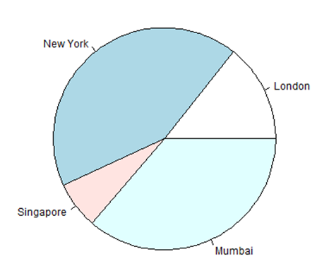
只使用输入向量和标签创建一个非常简单的饼图。 下面的脚本将在当前的R工作目录中创建并保存饼图。
# Create data for the graph.
x <- c(21, 62, 10, 53)
labels <- c("London", "New York", "Singapore", "Mumbai")
# Give the chart file a name.
png(file = "city.jpg")
# Plot the chart.
pie(x,labels)
# Save the file.
dev.off()
当我们执行上面的代码时,它会产生以下结果 -
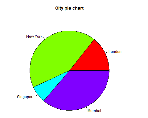
饼图标题和颜色
我们可以通过向函数添加更多参数来扩展图表的功能。 我们将使用参数main为图表添加标题,另一个参数是col ,它将在绘制图表时使用彩虹色托盘。 托盘的长度应与图表的值相同。 因此我们使用长度(x)。
例子 (Example)
下面的脚本将在当前的R工作目录中创建并保存饼图。
# Create data for the graph.
x <- c(21, 62, 10, 53)
labels <- c("London", "New York", "Singapore", "Mumbai")
# Give the chart file a name.
png(file = "city_title_colours.jpg")
# Plot the chart with title and rainbow color pallet.
pie(x, labels, main = "City pie chart", col = rainbow(length(x)))
# Save the file.
dev.off()
当我们执行上面的代码时,它会产生以下结果 -
切片百分比和图表图例
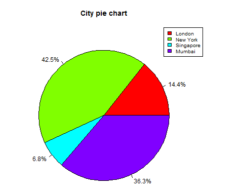
我们可以通过创建其他图表变量来添加切片百分比和图表图例。
# Create data for the graph.
x <- c(21, 62, 10,53)
labels <- c("London","New York","Singapore","Mumbai")
piepercent<- round(100*x/sum(x), 1)
# Give the chart file a name.
png(file = "city_percentage_legends.jpg")
# Plot the chart.
pie(x, labels = piepercent, main = "City pie chart",col = rainbow(length(x)))
legend("topright", c("London","New York","Singapore","Mumbai"), cex = 0.8,
fill = rainbow(length(x)))
# Save the file.
dev.off()
当我们执行上面的代码时,它会产生以下结果 -
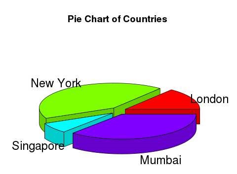
3D饼图
可以使用其他包绘制具有3个维度的饼图。 封装plotrix有一个名为pie3D()的函数用于此目的。
# Get the library.
library(plotrix)
# Create data for the graph.
x <- c(21, 62, 10,53)
lbl <- c("London","New York","Singapore","Mumbai")
# Give the chart file a name.
png(file = "3d_pie_chart.jpg")
# Plot the chart.
pie3D(x,labels = lbl,explode = 0.1, main = "Pie Chart of Countries ")
# Save the file.
dev.off()
当我们执行上面的代码时,它会产生以下结果 -
R - Bar Charts
条形图表示矩形条中的数据,条的长度与变量的值成比例。 R使用barplot()函数创建条形图。 R可以在条形图中绘制垂直条和水平条。 在条形图中,每个条形图可以被赋予不同的颜色。
语法 (Syntax)
在R中创建条形图的基本语法是 -
barplot(H,xlab,ylab,main, names.arg,col)
以下是所用参数的说明 -
- H是包含条形图中使用的数值的矢量或矩阵。
- xlab是x轴的标签。
- ylab是y轴的标签。
- main是条形图的标题。
- names.arg是出现在每个条形下的名称的向量。
- col用于为图形中的条形图提供颜色。
例子 (Example)
仅使用输入向量和每个条的名称创建简单的条形图。
以下脚本将在当前R工作目录中创建并保存条形图。
# Create the data for the chart
H <- c(7,12,28,3,41)
# Give the chart file a name
png(file = "barchart.png")
# Plot the bar chart
barplot(H)
# Save the file
dev.off()
当我们执行上面的代码时,它产生以下结果 -
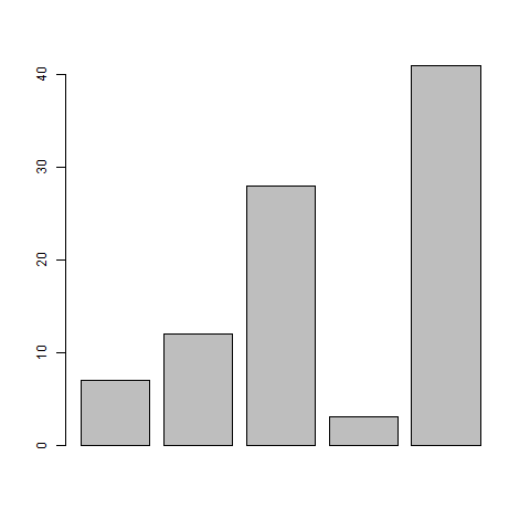
条形图标签,标题和颜色
可以通过添加更多参数来扩展条形图的功能。 main参数用于添加title 。 col参数用于向条形添加颜色。 args.name是具有与输入向量相同数量的值的向量,用于描述每个条的含义。
例子 (Example)
以下脚本将在当前R工作目录中创建并保存条形图。
# Create the data for the chart
H <- c(7,12,28,3,41)
M <- c("Mar","Apr","May","Jun","Jul")
# Give the chart file a name
png(file = "barchart_months_revenue.png")
# Plot the bar chart
barplot(H,names.arg=M,xlab="Month",ylab="Revenue",col="blue",
main="Revenue chart",border="red")
# Save the file
dev.off()
当我们执行上面的代码时,它产生以下结果 -
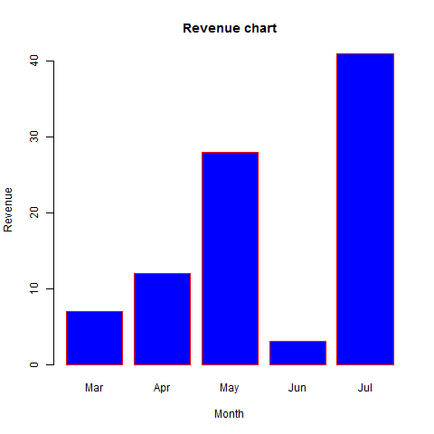
组条形图和堆积条形图
我们可以使用矩阵作为输入值,在每个条形图中创建条形图和堆栈组的条形图。
两个以上的变量表示为矩阵,用于创建组条形图和堆积条形图。
# Create the input vectors.
colors = c("green","orange","brown")
months <- c("Mar","Apr","May","Jun","Jul")
regions <- c("East","West","North")
# Create the matrix of the values.
Values <- matrix(c(2,9,3,11,9,4,8,7,3,12,5,2,8,10,11), nrow = 3, ncol = 5, byrow = TRUE)
# Give the chart file a name
png(file = "barchart_stacked.png")
# Create the bar chart
barplot(Values, main = "total revenue", names.arg = months, xlab = "month", ylab = "revenue", col = colours)
# Add the legend to the chart
legend("topleft", regions, cex = 1.3, fill = colours)
# Save the file
dev.off()
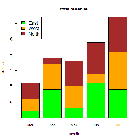
R - Boxplots
箱线图是衡量数据集中数据分布情况的指标。 它将数据集分为三个四分位数。 该图表示数据集中的最小值,最大值,中值,第一四分位数和第三四分位数。 通过为每个数据集绘制箱线图来比较数据集之间的数据分布也很有用。
通过使用boxplot boxplot()函数在R中创建boxplot() 。
语法 (Syntax)
在R中创建boxplot的基本语法是 -
boxplot(x, data, notch, varwidth, names, main)
以下是所用参数的说明 -
x是矢量或公式。
data是数据框。
notch是一个逻辑值。 设置为TRUE以绘制缺口。
varwidth是一个逻辑值。 设置为true以绘制与样本大小成比例的框的宽度。
names是将在每个箱线图下打印的组标签。
main用于给图形标题。
例子 (Example)
我们使用R环境中可用的数据集“mtcars”来创建基本的boxplot。 让我们看看mtcars中的列“mpg”和“cyl”。
input <- mtcars[,c('mpg','cyl')]
print(head(input))
当我们执行上面的代码时,它产生以下结果 -
mpg cyl
Mazda RX4 21.0 6
Mazda RX4 Wag 21.0 6
Datsun 710 22.8 4
Hornet 4 Drive 21.4 6
Hornet Sportabout 18.7 8
Valiant 18.1 6
创建Boxplot
下面的脚本将为mpg(每加仑英里数)和cyl(汽缸数)之间的关系创建一个箱线图。
# Give the chart file a name.
png(file = "boxplot.png")
# Plot the chart.
boxplot(mpg ~ cyl, data = mtcars, xlab = "Number of Cylinders",
ylab = "Miles Per Gallon", main = "Mileage Data")
# Save the file.
dev.off()
当我们执行上面的代码时,它会产生以下结果 -
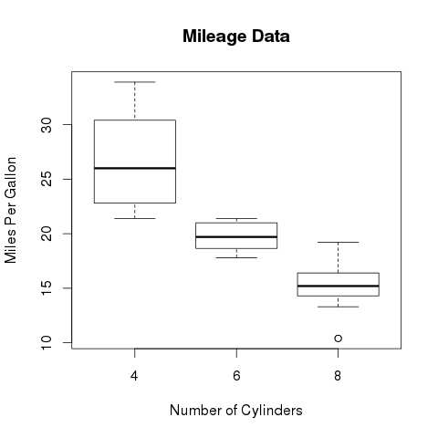
Boxplot与Notch
我们可以绘制带有缺口的boxplot,以了解不同数据组的中位数如何相互匹配。
下面的脚本将为每个数据组创建一个带有凹槽的箱线图。
# Give the chart file a name.
png(file = "boxplot_with_notch.png")
# Plot the chart.
boxplot(mpg ~ cyl, data = mtcars,
xlab = "Number of Cylinders",
ylab = "Miles Per Gallon",
main = "Mileage Data",
notch = TRUE,
varwidth = TRUE,
col = c("green","yellow","purple"),
names = c("High","Medium","Low")
)
# Save the file.
dev.off()
当我们执行上面的代码时,它会产生以下结果 -
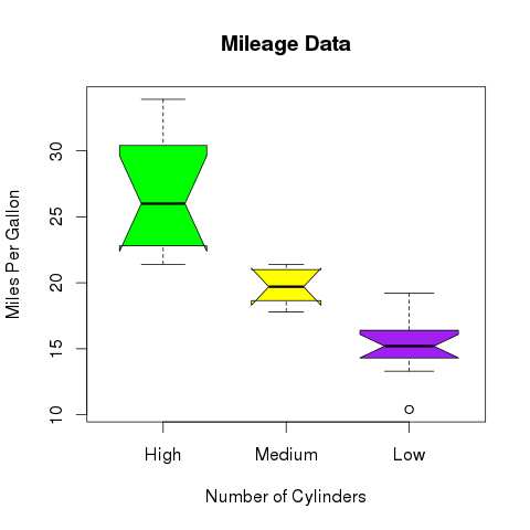
R - Histograms
直方图表示变换为范围的变量的值的频率。 直方图类似于条形聊天,但区别在于它将值分组为连续范围。 直方图中的每个条形表示该范围内存在的值的数量的高度。
R使用hist()函数创建直方图。 此函数将矢量作为输入,并使用一些更多参数来绘制直方图。
语法 (Syntax)
使用R创建直方图的基本语法是 -
hist(v,main,xlab,xlim,ylim,breaks,col,border)
以下是所用参数的说明 -
v是包含直方图中使用的数值的向量。
main表示图表的标题。
col用于设置条形的颜色。
border用于设置每个条的边框颜色。
xlab用于给出x轴的描述。
xlim用于指定x轴上的值范围。
ylim用于指定y轴上的值范围。
breaks用于提及每个条的宽度。
例子 (Example)
使用输入矢量,标签,col和边界参数创建简单的直方图。
下面给出的脚本将创建并保存当前R工作目录中的直方图。
# Create data for the graph.
v <- c(9,13,21,8,36,22,12,41,31,33,19)
# Give the chart file a name.
png(file = "histogram.png")
# Create the histogram.
hist(v,xlab = "Weight",col = "yellow",border = "blue")
# Save the file.
dev.off()
当我们执行上面的代码时,它会产生以下结果 -
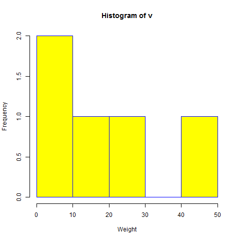
X和Y值的范围
要指定X轴和Y轴允许的值范围,我们可以使用xlim和ylim参数。
每个条的宽度可以通过使用休息来确定。
# Create data for the graph.
v <- c(9,13,21,8,36,22,12,41,31,33,19)
# Give the chart file a name.
png(file = "histogram_lim_breaks.png")
# Create the histogram.
hist(v,xlab = "Weight",col = "green",border = "red", xlim = c(0,40), ylim = c(0,5),
breaks = 5)
# Save the file.
dev.off()
当我们执行上面的代码时,它会产生以下结果 -
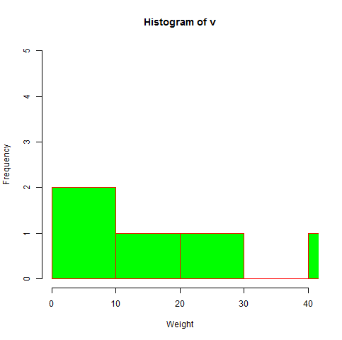
R - Line Graphs
折线图是通过在它们之间绘制线段来连接一系列点的图形。 这些点以其坐标(通常是x坐标)值之一排序。 折线图通常用于识别数据趋势。
R中的plot()函数用于创建折线图。
语法 (Syntax)
在R中创建折线图的基本语法是 -
plot(v,type,col,xlab,ylab)
以下是所用参数的说明 -
v是包含数值的向量。
type取值“p”只绘制点,“l”只绘制线,“o”绘制点和线。
xlab是x轴的标签。
ylab是y轴的标签。
main是图表的标题。
col用于为点和线提供颜色。
例子 (Example)
使用输入向量和类型参数“O”创建简单折线图。 下面的脚本将在当前的R工作目录中创建并保存折线图。
# Create the data for the chart.
v <- c(7,12,28,3,41)
# Give the chart file a name.
png(file = "line_chart.jpg")
# Plot the bar chart.
plot(v,type = "o")
# Save the file.
dev.off()
当我们执行上面的代码时,它会产生以下结果 -
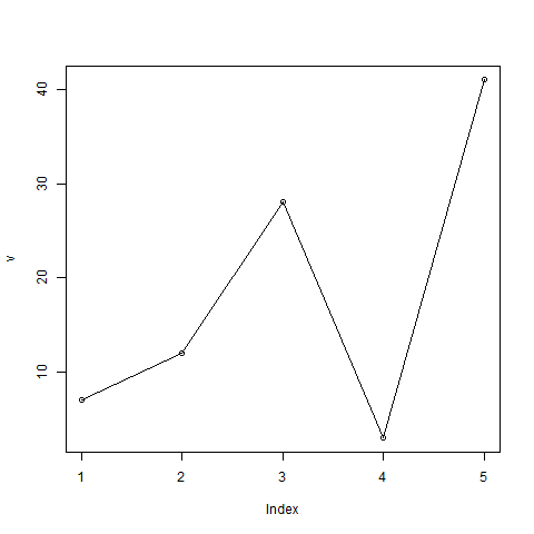
折线图标题,颜色和标签
可以使用其他参数扩展折线图的功能。 我们为点和线添加颜色,为图表添加标题并为轴添加标签。
例子 (Example)
# Create the data for the chart.
v <- c(7,12,28,3,41)
# Give the chart file a name.
png(file = "line_chart_label_colored.jpg")
# Plot the bar chart.
plot(v,type = "o", col = "red", xlab = "Month", ylab = "Rain fall",
main = "Rain fall chart")
# Save the file.
dev.off()
当我们执行上面的代码时,它会产生以下结果 -
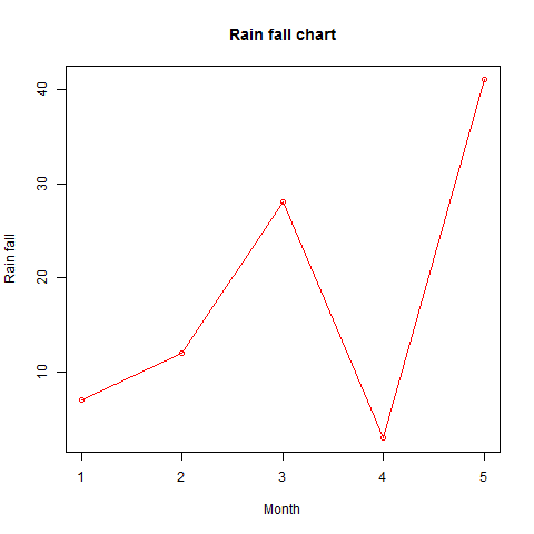
折线图中的多条线
通过使用lines()函数,可以在同一图表上绘制多lines() 。
绘制第一行后,lines()函数可以使用附加向量作为输入来绘制图表中的第二行,
# Create the data for the chart.
v <- c(7,12,28,3,41)
t <- c(14,7,6,19,3)
# Give the chart file a name.
png(file = "line_chart_2_lines.jpg")
# Plot the bar chart.
plot(v,type = "o",col = "red", xlab = "Month", ylab = "Rain fall",
main = "Rain fall chart")
lines(t, type = "o", col = "blue")
# Save the file.
dev.off()
当我们执行上面的代码时,它会产生以下结果 -
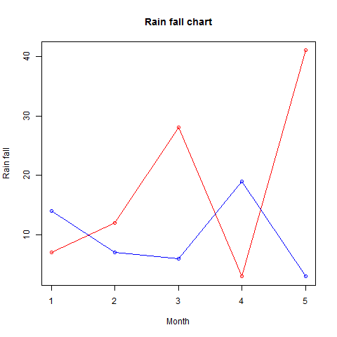
R - Scatterplots
散点图显示在笛卡尔平面中绘制的许多点。 每个点代表两个变量的值。 在水平轴上选择一个变量,在垂直轴上选择另一个变量。
使用plot()函数创建简单的散点图。
语法 (Syntax)
在R中创建散点图的基本语法是 -
plot(x, y, main, xlab, ylab, xlim, ylim, axes)
以下是所用参数的说明 -
x是数值集,其值是水平坐标。
y是数值集,其值是垂直坐标。
main是图的图块。
xlab是水平轴上的标签。
ylab是垂直轴上的标签。
xlim是用于绘图的x值的限制。
ylim是用于绘图的y值的极限。
axes表示是否应在绘图上绘制两个轴。
例子 (Example)
我们使用R环境中可用的数据集"mtcars"来创建基本散点图。 我们在mtcars中使用“wt”和“mpg”列。
input <- mtcars[,c('wt','mpg')]
print(head(input))
当我们执行上面的代码时,它会产生以下结果 -
wt mpg
Mazda RX4 2.620 21.0
Mazda RX4 Wag 2.875 21.0
Datsun 710 2.320 22.8
Hornet 4 Drive 3.215 21.4
Hornet Sportabout 3.440 18.7
Valiant 3.460 18.1
创建散点图
下面的脚本将为wt(重量)和mpg(每加仑英里数)之间的关系创建一个散点图。
# Get the input values.
input <- mtcars[,c('wt','mpg')]
# Give the chart file a name.
png(file = "scatterplot.png")
# Plot the chart for cars with weight between 2.5 to 5 and mileage between 15 and 30.
plot(x = input$wt,y = input$mpg,
xlab = "Weight",
ylab = "Milage",
xlim = c(2.5,5),
ylim = c(15,30),
main = "Weight vs Milage"
)
# Save the file.
dev.off()
当我们执行上面的代码时,它会产生以下结果 -
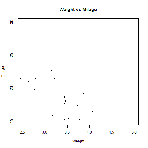
散点图矩阵
当我们有两个以上的变量并且我们想要找到一个变量与其余变量之间的相关性时,我们使用scatterplot矩阵。 我们使用pairs()函数来创建散点图的矩阵。
语法 (Syntax)
在R中创建散点图矩阵的基本语法是 -
pairs(formula, data)
以下是所用参数的说明 -
formula表示成对使用的一系列变量。
data表示将从中获取变量的数据集。
例子 (Example)
每个变量与剩余变量中的每一个配对。 绘制每对的散点图。
# Give the chart file a name.
png(file = "scatterplot_matrices.png")
# Plot the matrices between 4 variables giving 12 plots.
# One variable with 3 others and total 4 variables.
pairs(~wt+mpg+disp+cyl,data = mtcars,
main = "Scatterplot Matrix")
# Save the file.
dev.off()
执行上面的代码时,我们得到以下输出。
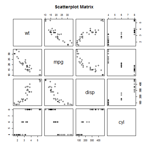
R - Mean, Median and Mode
R中的统计分析通过使用许多内置函数来执行。 大多数这些函数都是R基础包的一部分。 这些函数将R vector作为输入与参数一起使用并给出结果。
我们在本章讨论的函数是均值,中位数和模式。
Mean
它是通过取值的总和并除以数据系列中的值的数量来计算的。
函数mean()用于在R中计算。
语法 (Syntax)
计算R中均值的基本语法是 -
mean(x, trim = 0, na.rm = FALSE, ...)
以下是所用参数的说明 -
x是输入向量。
trim用于从排序向量的两端删除一些观察值。
na.rm用于从输入向量中删除缺失值。
例子 (Example)
# Create a vector.
x <- c(12,7,3,4.2,18,2,54,-21,8,-5)
# Find Mean.
result.mean <- mean(x)
print(result.mean)
当我们执行上面的代码时,它会产生以下结果 -
[1] 8.22
应用修剪选项
当提供trim参数时,向量中的值将被排序,然后从计算平均值中删除所需的观察数。
当trim = 0.3时,将从计算中删除每端的3个值以找到平均值。
在这种情况下,排序的向量是(-21,-5,2,3,4.2,7,8,12,18,54),从计算平均值的向量中删除的值是(-21,-5,2)从左边和(12,18,54)从右边。
# Create a vector.
x <- c(12,7,3,4.2,18,2,54,-21,8,-5)
# Find Mean.
result.mean <- mean(x,trim = 0.3)
print(result.mean)
当我们执行上面的代码时,它会产生以下结果 -
[1] 5.55
应用NA选项
如果存在缺失值,则均值函数返回NA。
要从计算中删除缺失值,请使用na.rm = TRUE。 这意味着删除NA值。
# Create a vector.
x <- c(12,7,3,4.2,18,2,54,-21,8,-5,NA)
# Find mean.
result.mean <- mean(x)
print(result.mean)
# Find mean dropping NA values.
result.mean <- mean(x,na.rm = TRUE)
print(result.mean)
当我们执行上面的代码时,它会产生以下结果 -
[1] NA
[1] 8.22
Median
数据系列中最中间的值称为中位数。 在R中使用median()函数来计算该值。
语法 (Syntax)
计算R中的中位数的基本语法是 -
median(x, na.rm = FALSE)
以下是所用参数的说明 -
x是输入向量。
na.rm用于从输入向量中删除缺失值。
例子 (Example)
# Create the vector.
x <- c(12,7,3,4.2,18,2,54,-21,8,-5)
# Find the median.
median.result <- median(x)
print(median.result)
当我们执行上面的代码时,它会产生以下结果 -
[1] 5.6
Mode
模式是一组数据中出现次数最多的值。 不一致的均值和中位数,模式可以同时具有数字和字符数据。
R没有标准的内置函数来计算模式。 因此,我们创建了一个用户函数来计算R中数据集的模式。该函数将向量作为输入,并将模式值作为输出。
例子 (Example)
# Create the function.
getmode <- function(v) {
uniqv <- unique(v)
uniqv[which.max(tabulate(match(v, uniqv)))]
}
# Create the vector with numbers.
v <- c(2,1,2,3,1,2,3,4,1,5,5,3,2,3)
# Calculate the mode using the user function.
result <- getmode(v)
print(result)
# Create the vector with characters.
charv <- c("o","it","the","it","it")
# Calculate the mode using the user function.
result <- getmode(charv)
print(result)
当我们执行上面的代码时,它会产生以下结果 -
[1] 2
[1] "it"
R - Linear Regression
回归分析是一种非常广泛使用的统计工具,用于建立两个变量之间的关系模型。 其中一个变量称为预测变量,其值通过实验收集。 另一个变量称为响应变量,其值来自预测变量。
在线性回归中,这两个变量通过等式相关,其中这两个变量的指数(幂)为1.数学上,线性关系表示绘制为图形时的直线。 任何变量的指数不等于1的非线性关系都会产生一条曲线。
线性回归的一般数学方程是 -
y = ax + b
以下是所用参数的说明 -
y是响应变量。
x是预测变量。
a和b是常量,称为系数。
建立回归的步骤
回归的一个简单例子是当人的身高已知时预测一个人的体重。 要做到这一点,我们需要有一个人的身高和体重之间的关系。
创建关系的步骤是 -
进行收集高度和相应重量观测值样本的实验。
使用R中的lm()函数创建关系模型
从创建的模型中查找系数,并使用这些系数创建数学方程
获取关系模型的摘要以了解预测中的平均误差。 也称为residuals 。
要预测新人的权重,请使用R中的predict()函数。
数据输入 (Input Data)
以下是代表观察结果的样本数据 -
# Values of height
151, 174, 138, 186, 128, 136, 179, 163, 152, 131
# Values of weight.
63, 81, 56, 91, 47, 57, 76, 72, 62, 48
lm() Function
此函数创建预测变量和响应变量之间的关系模型。
语法 (Syntax)
线性回归中lm()函数的基本语法是 -
lm(formula,data)
以下是所用参数的说明 -
formula是表示x和y之间关系的符号。
data是将应用公式的向量。
创建关系模型并获得系数
x <- c(151, 174, 138, 186, 128, 136, 179, 163, 152, 131)
y <- c(63, 81, 56, 91, 47, 57, 76, 72, 62, 48)
# Apply the lm() function.
relation <- lm(y~x)
print(relation)
当我们执行上面的代码时,它会产生以下结果 -
Call:
lm(formula = y ~ x)
Coefficients:
(Intercept) x
-38.4551 0.6746
获取关系摘要
x <- c(151, 174, 138, 186, 128, 136, 179, 163, 152, 131)
y <- c(63, 81, 56, 91, 47, 57, 76, 72, 62, 48)
# Apply the lm() function.
relation <- lm(y~x)
print(summary(relation))
当我们执行上面的代码时,它会产生以下结果 -
Call:
lm(formula = y ~ x)
Residuals:
Min 1Q Median 3Q Max
-6.3002 -1.6629 0.0412 1.8944 3.9775
Coefficients:
Estimate Std. Error t value Pr(>|t|)
(Intercept) -38.45509 8.04901 -4.778 0.00139 **
x 0.67461 0.05191 12.997 1.16e-06 ***
---
Signif. codes: 0 ‘***’ 0.001 ‘**’ 0.01 ‘*’ 0.05 ‘.’ 0.1 ‘ ’ 1
Residual standard error: 3.253 on 8 degrees of freedom
Multiple R-squared: 0.9548, Adjusted R-squared: 0.9491
F-statistic: 168.9 on 1 and 8 DF, p-value: 1.164e-06
predict() Function
语法 (Syntax)
线性回归中predict()的基本语法是 -
predict(object, newdata)
以下是所用参数的说明 -
object是已使用lm()函数创建的公式。
newdata是包含预测变量的新值的向量。
预测新人的重量
# The predictor vector.
x <- c(151, 174, 138, 186, 128, 136, 179, 163, 152, 131)
# The resposne vector.
y <- c(63, 81, 56, 91, 47, 57, 76, 72, 62, 48)
# Apply the lm() function.
relation <- lm(y~x)
# Find weight of a person with height 170.
a <- data.frame(x = 170)
result <- predict(relation,a)
print(result)
当我们执行上面的代码时,它会产生以下结果 -
1
76.22869
以图形方式显示回归
# Create the predictor and response variable.
x <- c(151, 174, 138, 186, 128, 136, 179, 163, 152, 131)
y <- c(63, 81, 56, 91, 47, 57, 76, 72, 62, 48)
relation <- lm(y~x)
# Give the chart file a name.
png(file = "linearregression.png")
# Plot the chart.
plot(y,x,col = "blue",main = "Height & Weight Regression",
abline(lm(x~y)),cex = 1.3,pch = 16,xlab = "Weight in Kg",ylab = "Height in cm")
# Save the file.
dev.off()
当我们执行上面的代码时,它会产生以下结果 -
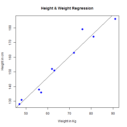
R - Multiple Regression
多元回归是线性回归到两个以上变量之间关系的扩展。 在简单线性关系中,我们有一个预测变量和一个响应变量,但在多元回归中,我们有多个预测变量和一个响应变量。
多元回归的一般数学方程是 -
y = a + b1x1 + b2x2 +...bnxn
以下是所用参数的说明 -
y是响应变量。
a, b1, b2...bn是系数。
x1, x2, ...xn是预测变量。
我们使用R中的lm()函数创建回归模型。模型使用输入数据确定系数的值。 接下来,我们可以使用这些系数预测给定预测变量集的响应变量的值。
lm() Function
此函数创建预测变量和响应变量之间的关系模型。
语法 (Syntax)
多元回归中lm()函数的基本语法是 -
lm(y ~ x1+x2+x3...,data)
以下是所用参数的说明 -
formula是表示响应变量和预测变量之间关系的符号。
data是将应用公式的向量。
例子 (Example)
数据输入 (Input Data)
考虑R环境中可用的数据集“mtcars”。 它给出了不同车型在每加仑行驶里程(mpg),汽缸排量(“disp”),马力(“hp”),汽车重量(“wt”)和更多参数方面的比较。
该模型的目标是建立“mpg”作为响应变量与“disp”,“hp”和“wt”之间的关系作为预测变量。 为此,我们从mtcars数据集中创建这些变量的子集。
input <- mtcars[,c("mpg","disp","hp","wt")]
print(head(input))
当我们执行上面的代码时,它会产生以下结果 -
mpg disp hp wt
Mazda RX4 21.0 160 110 2.620
Mazda RX4 Wag 21.0 160 110 2.875
Datsun 710 22.8 108 93 2.320
Hornet 4 Drive 21.4 258 110 3.215
Hornet Sportabout 18.7 360 175 3.440
Valiant 18.1 225 105 3.460
创建关系模型并获得系数
input <- mtcars[,c("mpg","disp","hp","wt")]
# Create the relationship model.
model <- lm(mpg~disp+hp+wt, data = input)
# Show the model.
print(model)
# Get the Intercept and coefficients as vector elements.
cat("# # # # The Coefficient Values # # # ","\n")
a <- coef(model)[1]
print(a)
Xdisp <- coef(model)[2]
Xhp <- coef(model)[3]
Xwt <- coef(model)[4]
print(Xdisp)
print(Xhp)
print(Xwt)
当我们执行上面的代码时,它会产生以下结果 -
Call:
lm(formula = mpg ~ disp + hp + wt, data = input)
Coefficients:
(Intercept) disp hp wt
37.105505 -0.000937 -0.031157 -3.800891
# # # # The Coefficient Values # # #
(Intercept)
37.10551
disp
-0.0009370091
hp
-0.03115655
wt
-3.800891
创建回归模型的方程
基于上述截距和系数值,我们创建了数学方程。
Y = a+Xdisp.x1+Xhp.x2+Xwt.x3
or
Y = 37.15+(-0.000937)*x1+(-0.0311)*x2+(-3.8008)*x3
应用公式来预测新值
我们可以使用上面创建的回归方程来预测一组新的位移,马力和重量值时的里程数。
对于disp = 221,hp = 102且wt = 2.91的汽车,预计里程为 -
Y = 37.15+(-0.000937)*221+(-0.0311)*102+(-3.8008)*2.91 = 22.7104
R - Logistic Regression
Logistic回归是一种回归模型,其中响应变量(因变量)具有分类值,例如True/False或0/1。 它实际上基于将其与预测变量相关联的数学方程来测量二元响应的概率作为响应变量的值。
逻辑回归的一般数学方程是 -
y = 1/(1+e^-(a+b1x1+b2x2+b3x3+...))
以下是所用参数的说明 -
y是响应变量。
x是预测变量。
a和b是数值常数的系数。
用于创建回归模型的函数是glm()函数。
语法 (Syntax)
逻辑回归中glm()函数的基本语法是 -
glm(formula,data,family)
以下是所用参数的说明 -
formula是表示变量之间关系的符号。
data是给出这些变量值的数据集。
family是R对象,用于指定模型的详细信息。 对于逻辑回归,它的值是二项式的。
例子 (Example)
内置数据集“mtcars”描述了具有各种发动机规格的汽车的不同型号。 在“mtcars”数据集中,传输模式(自动或手动)由列am描述,其为二进制值(0或1)。 我们可以在列“am”和其他3列(hp,wt和cyl)之间创建逻辑回归模型。
# Select some columns form mtcars.
input <- mtcars[,c("am","cyl","hp","wt")]
print(head(input))
当我们执行上面的代码时,它会产生以下结果 -
am cyl hp wt
Mazda RX4 1 6 110 2.620
Mazda RX4 Wag 1 6 110 2.875
Datsun 710 1 4 93 2.320
Hornet 4 Drive 0 6 110 3.215
Hornet Sportabout 0 8 175 3.440
Valiant 0 6 105 3.460
创建回归模型
我们使用glm()函数创建回归模型并获得其摘要以供分析。
input <- mtcars[,c("am","cyl","hp","wt")]
am.data = glm(formula = am ~ cyl + hp + wt, data = input, family = binomial)
print(summary(am.data))
当我们执行上面的代码时,它会产生以下结果 -
Call:
glm(formula = am ~ cyl + hp + wt, family = binomial, data = input)
Deviance Residuals:
Min 1Q Median 3Q Max
-2.17272 -0.14907 -0.01464 0.14116 1.27641
Coefficients:
Estimate Std. Error z value Pr(>|z|)
(Intercept) 19.70288 8.11637 2.428 0.0152 *
cyl 0.48760 1.07162 0.455 0.6491
hp 0.03259 0.01886 1.728 0.0840 .
wt -9.14947 4.15332 -2.203 0.0276 *
---
Signif. codes: 0 ‘***’ 0.001 ‘**’ 0.01 ‘*’ 0.05 ‘.’ 0.1 ‘ ’ 1
(Dispersion parameter for binomial family taken to be 1)
Null deviance: 43.2297 on 31 degrees of freedom
Residual deviance: 9.8415 on 28 degrees of freedom
AIC: 17.841
Number of Fisher Scoring iterations: 8
结论 (Conclusion)
在摘要中,对于变量“cyl”和“hp”,最后一列中的p值大于0.05,我们认为它们对变量“am”的值有贡献是无关紧要的。 只有权重(wt)会影响此回归模型中的“am”值。
R - Normal Distribution
在来自独立来源的随机数据集中,通常观察到数据的分布是正常的。 这意味着,在绘制具有水平轴中变量值的图形和垂直轴中的值的计数时,我们得到钟形曲线。 曲线的中心表示数据集的平均值。 在图中,百分之五十的值位于均值的左侧,另外百分之五十位于图的右侧。 这在统计学中称为正态分布。
R有四个内置函数来生成正态分布。 它们如下所述。
dnorm(x, mean, sd)
pnorm(x, mean, sd)
qnorm(p, mean, sd)
rnorm(n, mean, sd)
以下是上述功能中使用的参数的说明 -
x是数字的向量。
p是概率的向量。
n是观察次数(样本量)。
mean是样本数据的平均值。 它的默认值为零。
sd是标准偏差。 它的默认值是1。
dnorm()
对于给定的平均值和标准偏差,此函数给出每个点处的概率分布的高度。
# Create a sequence of numbers between -10 and 10 incrementing by 0.1.
x <- seq(-10, 10, by = .1)
# Choose the mean as 2.5 and standard deviation as 0.5.
y <- dnorm(x, mean = 2.5, sd = 0.5)
# Give the chart file a name.
png(file = "dnorm.png")
plot(x,y)
# Save the file.
dev.off()
当我们执行上面的代码时,它会产生以下结果 -
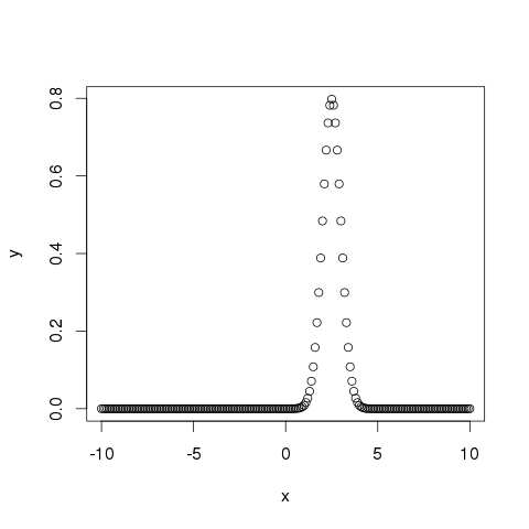
pnorm()
此函数给出正态分布随机数的概率小于给定数字的值。 它也被称为“累积分布函数”。
# Create a sequence of numbers between -10 and 10 incrementing by 0.2.
x <- seq(-10,10,by = .2)
# Choose the mean as 2.5 and standard deviation as 2.
y <- pnorm(x, mean = 2.5, sd = 2)
# Give the chart file a name.
png(file = "pnorm.png")
# Plot the graph.
plot(x,y)
# Save the file.
dev.off()
当我们执行上面的代码时,它会产生以下结果 -
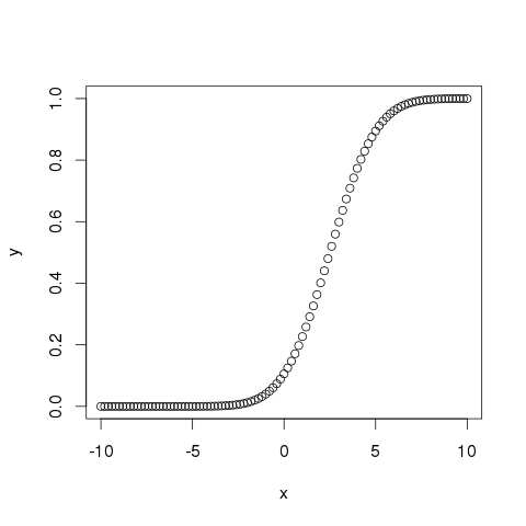
qnorm()
此函数获取概率值并给出其累积值与概率值匹配的数字。
# Create a sequence of probability values incrementing by 0.02.
x <- seq(0, 1, by = 0.02)
# Choose the mean as 2 and standard deviation as 3.
y <- qnorm(x, mean = 2, sd = 1)
# Give the chart file a name.
png(file = "qnorm.png")
# Plot the graph.
plot(x,y)
# Save the file.
dev.off()
当我们执行上面的代码时,它会产生以下结果 -
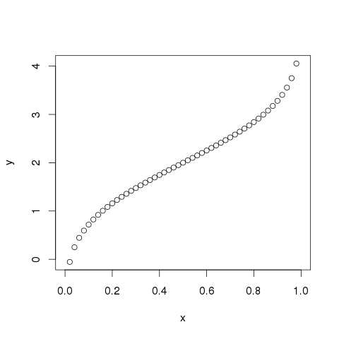
rnorm()
此函数用于生成分布正常的随机数。 它将样本大小作为输入并生成许多随机数。 我们绘制直方图以显示生成的数字的分布。
# Create a sample of 50 numbers which are normally distributed.
y <- rnorm(50)
# Give the chart file a name.
png(file = "rnorm.png")
# Plot the histogram for this sample.
hist(y, main = "Normal DIstribution")
# Save the file.
dev.off()
当我们执行上面的代码时,它会产生以下结果 -
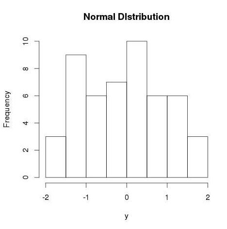
R - Binomial Distribution
二项分布模型用于找出事件成功的概率,该事件在一系列实验中仅具有两种可能的结果。 例如,投掷硬币总是给出头部或尾部。 在二项分布期间估计在重复投掷硬币10次时准确找到3个头的概率。
R有四个内置函数来生成二项分布。 它们如下所述。
dbinom(x, size, prob)
pbinom(x, size, prob)
qbinom(p, size, prob)
rbinom(n, size, prob)
以下是所用参数的说明 -
x是数字的向量。
p是概率的向量。
n是观察次数。
size是试验次数。
prob是每次试验成功的概率。
dbinom()
该函数给出了每个点的概率密度分布。
# Create a sample of 50 numbers which are incremented by 1.
x <- seq(0,50,by = 1)
# Create the binomial distribution.
y <- dbinom(x,50,0.5)
# Give the chart file a name.
png(file = "dbinom.png")
# Plot the graph for this sample.
plot(x,y)
# Save the file.
dev.off()
当我们执行上面的代码时,它会产生以下结果 -
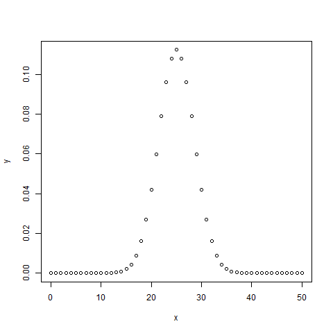
pbinom()
此函数给出事件的累积概率。 它是表示概率的单个值。
# Probability of getting 26 or less heads from a 51 tosses of a coin.
x <- pbinom(26,51,0.5)
print(x)
当我们执行上面的代码时,它会产生以下结果 -
[1] 0.610116
qbinom()
此函数获取概率值并给出其累积值与概率值匹配的数字。
# How many heads will have a probability of 0.25 will come out when a coin
# is tossed 51 times.
x <- qbinom(0.25,51,1/2)
print(x)
当我们执行上面的代码时,它会产生以下结果 -
[1] 23
rbinom()
此函数从给定样本生成给定概率的所需数量的随机值。
# Find 8 random values from a sample of 150 with probability of 0.4.
x <- rbinom(8,150,.4)
print(x)
当我们执行上面的代码时,它会产生以下结果 -
[1] 58 61 59 66 55 60 61 67
R - Poisson Regression
泊松回归涉及回归模型,其中响应变量是计数而不是分数的形式。 例如,足球比赛系列中的出生人数或获胜次数。 此外,响应变量的值遵循泊松分布。
泊松回归的一般数学方程是 -
log(y) = a + b1x1 + b2x2 + bnxn.....
以下是所用参数的说明 -
y是响应变量。
a和b是数字系数。
x是预测变量。
用于创建泊松回归模型的函数是glm()函数。
语法 (Syntax)
泊松回归中glm()函数的基本语法是 -
glm(formula,data,family)
以下是上述功能中使用的参数的说明 -
formula是表示变量之间关系的符号。
data是给出这些变量值的数据集。
family是R对象,用于指定模型的详细信息。 它的值是Logistic回归的“泊松”。
例子 (Example)
我们有内置的数据集“warpbreaks”,它描述了羊毛类型(A或B)和张力(低,中或高)对每个织机经纱断裂次数的影响。 让我们将“break”视为响应变量,它是一个中断次数的计数。 羊毛“类型”和“张力”被视为预测变量。
Input Data
input <- warpbreaks
print(head(input))
当我们执行上面的代码时,它会产生以下结果 -
breaks wool tension
1 26 A L
2 30 A L
3 54 A L
4 25 A L
5 70 A L
6 52 A L
创建回归模型
output <-glm(formula = breaks ~ wool+tension, data = warpbreaks,
family = poisson)
print(summary(output))
当我们执行上面的代码时,它会产生以下结果 -
Call:
glm(formula = breaks ~ wool + tension, family = poisson, data = warpbreaks)
Deviance Residuals:
Min 1Q Median 3Q Max
-3.6871 -1.6503 -0.4269 1.1902 4.2616
Coefficients:
Estimate Std. Error z value Pr(>|z|)
(Intercept) 3.69196 0.04541 81.302 < 2e-16 ***
woolB -0.20599 0.05157 -3.994 6.49e-05 ***
tensionM -0.32132 0.06027 -5.332 9.73e-08 ***
tensionH -0.51849 0.06396 -8.107 5.21e-16 ***
---
Signif. codes: 0 ‘***’ 0.001 ‘**’ 0.01 ‘*’ 0.05 ‘.’ 0.1 ‘ ’ 1
(Dispersion parameter for poisson family taken to be 1)
Null deviance: 297.37 on 53 degrees of freedom
Residual deviance: 210.39 on 50 degrees of freedom
AIC: 493.06
Number of Fisher Scoring iterations: 4
在摘要中,我们寻找最后一列中的p值小于0.05,以考虑预测变量对响应变量的影响。 如图所示,具有M型和H型张力的羊毛B对断裂次数有影响。
R - Analysis of Covariance
我们使用回归分析来创建描述预测变量的变化对响应变量的影响的模型。 有时,如果我们有一个分类变量,其值为Yes/No或Male/Female等。简单回归分析为分类变量的每个值提供多个结果。 在这种情况下,我们可以通过将分类变量与预测变量一起使用并比较分类变量的每个级别的回归线来研究分类变量的影响。 这种分析被称为Analysis of Covariance也称为ANCOVA 。
例子 (Example)
考虑R内置的数据集mtcars。 在其中我们观察到“am”字段代表传输类型(自动或手动)。 它是一个值为0和1的分类变量。除了马力值(“hp”)之外,汽车的每加仑英里数(mpg)也可以取决于它。
我们研究“am”的值对“mpg”和“hp”之间的回归的影响。 这是通过使用aov()函数,然后使用aov() anova()函数来比较多个回归来完成的。
输入数据 (Input Data)
从数据集mtcars创建一个包含字段“mpg”,“hp”和“am”的数据框。 这里我们将“mpg”作为响应变量,“hp”作为预测变量,“am”作为分类变量。
input <- mtcars[,c("am","mpg","hp")]
print(head(input))
当我们执行上面的代码时,它会产生以下结果 -
am mpg hp
Mazda RX4 1 21.0 110
Mazda RX4 Wag 1 21.0 110
Datsun 710 1 22.8 93
Hornet 4 Drive 0 21.4 110
Hornet Sportabout 0 18.7 175
Valiant 0 18.1 105
ANCOVA分析
我们创建一个回归模型,将“hp”作为预测变量,将“mpg”作为响应变量,同时考虑“am”和“hp”之间的相互作用。
具有分类变量和预测变量之间相互作用的模型
# Get the dataset.
input <- mtcars
# Create the regression model.
result <- aov(mpg~hp*am,data = input)
print(summary(result))
当我们执行上面的代码时,它会产生以下结果 -
Df Sum Sq Mean Sq F value Pr(>F)
hp 1 678.4 678.4 77.391 1.50e-09 ***
am 1 202.2 202.2 23.072 4.75e-05 ***
hp:am 1 0.0 0.0 0.001 0.981
Residuals 28 245.4 8.8
---
Signif. codes: 0 ‘***’ 0.001 ‘**’ 0.01 ‘*’ 0.05 ‘.’ 0.1 ‘ ’ 1
该结果表明,马力和传动类型对每加仑英里数有显着影响,因为两种情况下的p值均小于0.05。 但是这两个变量之间的相互作用并不显着,因为p值大于0.05。
模型没有分类变量和预测变量之间的相互作用
# Get the dataset.
input <- mtcars
# Create the regression model.
result <- aov(mpg~hp+am,data = input)
print(summary(result))
当我们执行上面的代码时,它会产生以下结果 -
Df Sum Sq Mean Sq F value Pr(>F)
hp 1 678.4 678.4 80.15 7.63e-10 ***
am 1 202.2 202.2 23.89 3.46e-05 ***
Residuals 29 245.4 8.5
---
Signif. codes: 0 ‘***’ 0.001 ‘**’ 0.01 ‘*’ 0.05 ‘.’ 0.1 ‘ ’ 1
该结果表明,马力和传动类型对每加仑英里数有显着影响,因为两种情况下的p值均小于0.05。
比较两种模型
现在我们可以比较两个模型,以得出变量的相互作用是否真正重要。 为此,我们使用anova()函数。
# Get the dataset.
input <- mtcars
# Create the regression models.
result1 <- aov(mpg~hp*am,data = input)
result2 <- aov(mpg~hp+am,data = input)
# Compare the two models.
print(anova(result1,result2))
当我们执行上面的代码时,它会产生以下结果 -
Model 1: mpg ~ hp * am
Model 2: mpg ~ hp + am
Res.Df RSS Df Sum of Sq F Pr(>F)
1 28 245.43
2 29 245.44 -1 -0.0052515 6e-04 0.9806
当p值大于0.05时,我们得出结论:马力和传递类型之间的相互作用并不显着。 因此,在汽车和手动变速器模式下,每加仑的里程数将以类似的方式取决于汽车的马力。
R - Time Series Analysis
时间序列是一系列数据点,其中每个数据点与时间戳相关联。 一个简单的例子是股票市场中某一天的不同时间点的股票价格。 另一个例子是一年中不同月份的一个地区的降雨量。 R语言使用许多函数来创建,操作和绘制时间序列数据。 时间序列的数据存储在称为time-series object的R time-series object 。 它也是一个R数据对象,如矢量或数据帧。
时间序列对象是使用ts()函数创建的。
语法 (Syntax)
时间序列分析中ts()函数的基本语法是 -
timeseries.object.name <- ts(data, start, end, frequency)
以下是所用参数的说明 -
data是包含时间序列中使用的值的向量或矩阵。
start指定时间序列中第一次观察的开始时间。
end指定时间序列中最后一次观察的结束时间。
frequency指定每单位时间的观测数量。
除参数“data”外,所有其他参数均为可选参数。
例子 (Example)
从2012年1月开始考虑一个地方的年降雨量详细信息。我们创建一个R时间序列对象,为期12个月并绘制它。
# Get the data points in form of a R vector.
rainfall <- c(799,1174.8,865.1,1334.6,635.4,918.5,685.5,998.6,784.2,985,882.8,1071)
# Convert it to a time series object.
rainfall.timeseries <- ts(rainfall,start = c(2012,1),frequency = 12)
# Print the timeseries data.
print(rainfall.timeseries)
# Give the chart file a name.
png(file = "rainfall.png")
# Plot a graph of the time series.
plot(rainfall.timeseries)
# Save the file.
dev.off()
当我们执行上面的代码时,它会产生以下结果和图表 -
Jan Feb Mar Apr May Jun Jul Aug Sep
2012 799.0 1174.8 865.1 1334.6 635.4 918.5 685.5 998.6 784.2
Oct Nov Dec
2012 985.0 882.8 1071.0
时间序列图表 -
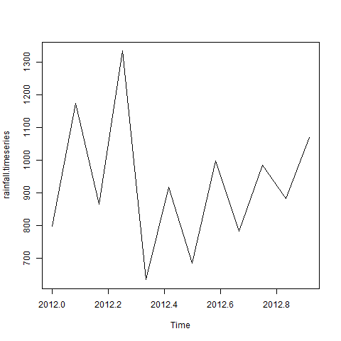
不同的时间间隔
ts()函数中frequency参数的值决定了测量数据点的时间间隔。 值12表示时间序列为12个月。 其他值及其含义如下 -
frequency = 12钉住一年中每个月的数据点。
frequency = 4每一季度的数据点。
frequency = 6每小时10分钟的数据点。
frequency = 24*6每天每10分钟固定数据点。
多个时间序列
我们可以通过将两个系列组合成一个矩阵,在一个图表中绘制多个时间序列。
# Get the data points in form of a R vector.
rainfall1 <- c(799,1174.8,865.1,1334.6,635.4,918.5,685.5,998.6,784.2,985,882.8,1071)
rainfall2 <-
c(655,1306.9,1323.4,1172.2,562.2,824,822.4,1265.5,799.6,1105.6,1106.7,1337.8)
# Convert them to a matrix.
combined.rainfall <- matrix(c(rainfall1,rainfall2),nrow = 12)
# Convert it to a time series object.
rainfall.timeseries <- ts(combined.rainfall,start = c(2012,1),frequency = 12)
# Print the timeseries data.
print(rainfall.timeseries)
# Give the chart file a name.
png(file = "rainfall_combined.png")
# Plot a graph of the time series.
plot(rainfall.timeseries, main = "Multiple Time Series")
# Save the file.
dev.off()
当我们执行上面的代码时,它会产生以下结果和图表 -
Series 1 Series 2
Jan 2012 799.0 655.0
Feb 2012 1174.8 1306.9
Mar 2012 865.1 1323.4
Apr 2012 1334.6 1172.2
May 2012 635.4 562.2
Jun 2012 918.5 824.0
Jul 2012 685.5 822.4
Aug 2012 998.6 1265.5
Sep 2012 784.2 799.6
Oct 2012 985.0 1105.6
Nov 2012 882.8 1106.7
Dec 2012 1071.0 1337.8
多时间系列图表 -
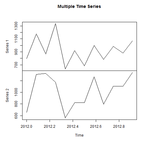
R - Nonlinear Least Square
在对真实世界数据进行建模以进行回归分析时,我们观察到模型方程很少是给出线性图的线性方程。 大多数情况下,现实世界数据模型的方程涉及更高程度的数学函数,如指数为3或sin函数。 在这种情况下,模型的图给出曲线而不是线。 线性回归和非线性回归的目标是调整模型参数的值,以找到最接近数据的直线或曲线。 在找到这些值后,我们将能够以良好的准确度估计响应变量。
在最小二乘回归中,我们建立一个回归模型,其中不同点与回归曲线的垂直距离的平方和最小。 我们通常从定义的模型开始并假设系数的一些值。 然后,我们应用R的nls()函数来获得更准确的值以及置信区间。
语法 (Syntax)
在R中创建非线性最小二乘检验的基本语法是 -
nls(formula, data, start)
以下是所用参数的说明 -
formula是包含变量和参数的非线性模型公式。
data是用于评估公式中变量的数据框。
start是一个命名列表或起始估计的命名数字向量。
例子 (Example)
我们将考虑一个假设其系数初始值的非线性模型。 接下来,我们将看到这些假设值的置信区间是什么,以便我们可以判断这些值对模型的影响程度。
所以让我们为此目的考虑下面的等式 -
a = b1*x^2+b2
假设初始系数为1和3,并将这些值拟合到nls()函数中。
xvalues <- c(1.6,2.1,2,2.23,3.71,3.25,3.4,3.86,1.19,2.21)
yvalues <- c(5.19,7.43,6.94,8.11,18.75,14.88,16.06,19.12,3.21,7.58)
# Give the chart file a name.
png(file = "nls.png")
# Plot these values.
plot(xvalues,yvalues)
# Take the assumed values and fit into the model.
model <- nls(yvalues ~ b1*xvalues^2+b2,start = list(b1 = 1,b2 = 3))
# Plot the chart with new data by fitting it to a prediction from 100 data points.
new.data <- data.frame(xvalues = seq(min(xvalues),max(xvalues),len = 100))
lines(new.data$xvalues,predict(model,newdata = new.data))
# Save the file.
dev.off()
# Get the sum of the squared residuals.
print(sum(resid(model)^2))
# Get the confidence intervals on the chosen values of the coefficients.
print(confint(model))
当我们执行上面的代码时,它会产生以下结果 -
[1] 1.081935
Waiting for profiling to be done...
2.5% 97.5%
b1 1.137708 1.253135
b2 1.497364 2.496484
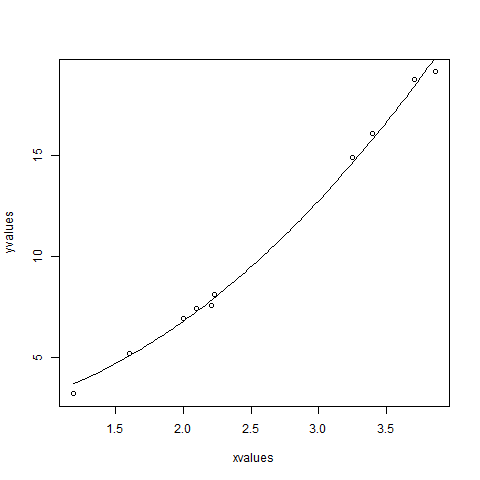
我们可以得出结论,b1的值更接近于1,而b2的值更接近2而不是3。
R - Decision Tree
决策树是以树的形式表示选择及其结果的图。 图中的节点表示事件或选择,图的边表示决策规则或条件。 它主要用于使用R的机器学习和数据挖掘应用程序。
使用决策树的例子是 - 将电子邮件预测为垃圾邮件或不垃圾邮件,预测肿瘤是癌症,或根据每个因素中的因素预测贷款是好的还是坏的信用风险。 通常,使用也称为训练数据的观察数据创建模型。 然后使用一组验证数据来验证和改进模型。 R具有用于创建和可视化决策树的包。 对于新的预测变量集,我们使用此模型来确定数据的类别(是/否,垃圾邮件/非垃圾邮件)。
R包"party"用于创建决策树。
安装R包
在R控制台中使用以下命令安装程序包。 您还必须安装依赖包(如果有)。
install.packages("party")
包“party”具有函数ctree() ,用于创建和分析decison树。
语法 (Syntax)
在R中创建决策树的基本语法是 -
ctree(formula, data)
以下是所用参数的说明 -
formula是描述预测变量和响应变量的公式。
data是使用的数据集的名称。
数据输入 (Input Data)
我们将使用名为readingSkills的R内置数据集来创建决策树。 如果我们知道变量“年龄”,“鞋子大小”,“得分”以及该人是否是母语者,它会描述某人阅读技能的分数。
这是样本数据。
# Load the party package. It will automatically load other
# dependent packages.
library(party)
# Print some records from data set readingSkills.
print(head(readingSkills))
当我们执行上面的代码时,它会产生以下结果和图表 -
nativeSpeaker age shoeSize score
1 yes 5 24.83189 32.29385
2 yes 6 25.95238 36.63105
3 no 11 30.42170 49.60593
4 yes 7 28.66450 40.28456
5 yes 11 31.88207 55.46085
6 yes 10 30.07843 52.83124
Loading required package: methods
Loading required package: grid
...............................
...............................
例子 (Example)
我们将使用ctree()函数创建决策树并查看其图形。
# Load the party package. It will automatically load other
# dependent packages.
library(party)
# Create the input data frame.
input.dat <- readingSkills[c(1:105),]
# Give the chart file a name.
png(file = "decision_tree.png")
# Create the tree.
output.tree <- ctree(
nativeSpeaker ~ age + shoeSize + score,
data = input.dat)
# Plot the tree.
plot(output.tree)
# Save the file.
dev.off()
当我们执行上面的代码时,它会产生以下结果 -
null device
1
Loading required package: methods
Loading required package: grid
Loading required package: mvtnorm
Loading required package: modeltools
Loading required package: stats4
Loading required package: strucchange
Loading required package: zoo
Attaching package: ‘zoo’
The following objects are masked from ‘package:base’:
as.Date, as.Date.numeric
Loading required package: sandwich
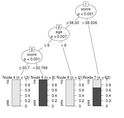
结论 (Conclusion)
从上面显示的决策树中我们可以得出结论,任何阅读技能得分低于38.3且年龄超过6的人都不是本地议长。
R - Random Forest
在随机森林方法中,创建了大量决策树。 每个观察都被送入每个决策树。 每次观察的最常见结果用作最终输出。 一个新的观察结果被输入所有树木,并对每个分类模型进行多数投票。
对构建树时未使用的情况进行错误估计。 这称为OOB (Out-of-bag)错误估计,以百分比形式提及。
R包"randomForest"用于创建随机森林。
安装R包
在R控制台中使用以下命令安装程序包。 您还必须安装依赖包(如果有)。
install.packages("randomForest)
包“randomForest”具有randomForest()函数,用于创建和分析随机森林。
语法 (Syntax)
在R中创建随机林的基本语法是 -
randomForest(formula, data)
以下是所用参数的说明 -
formula是描述预测变量和响应变量的公式。
data是使用的数据集的名称。
数据输入 (Input Data)
我们将使用名为readingSkills的R内置数据集来创建决策树。 如果我们知道变量“年龄”,“鞋子大小”,“得分”以及该人是否是母语人士,它会描述某人阅读技能的得分。
这是样本数据。
# Load the party package. It will automatically load other
# required packages.
library(party)
# Print some records from data set readingSkills.
print(head(readingSkills))
当我们执行上面的代码时,它会产生以下结果和图表 -
nativeSpeaker age shoeSize score
1 yes 5 24.83189 32.29385
2 yes 6 25.95238 36.63105
3 no 11 30.42170 49.60593
4 yes 7 28.66450 40.28456
5 yes 11 31.88207 55.46085
6 yes 10 30.07843 52.83124
Loading required package: methods
Loading required package: grid
...............................
...............................
例子 (Example)
我们将使用randomForest()函数来创建决策树并查看它的图形。
# Load the party package. It will automatically load other
# required packages.
library(party)
library(randomForest)
# Create the forest.
output.forest <- randomForest(nativeSpeaker ~ age + shoeSize + score,
data = readingSkills)
# View the forest results.
print(output.forest)
# Importance of each predictor.
print(importance(fit,type = 2))
当我们执行上面的代码时,它会产生以下结果 -
Call:
randomForest(formula = nativeSpeaker ~ age + shoeSize + score,
data = readingSkills)
Type of random forest: classification
Number of trees: 500
No. of variables tried at each split: 1
OOB estimate of error rate: 1%
Confusion matrix:
no yes class.error
no 99 1 0.01
yes 1 99 0.01
MeanDecreaseGini
age 13.95406
shoeSize 18.91006
score 56.73051
结论 (Conclusion)
从上面显示的随机森林我们可以得出结论,鞋子和分数是决定某人是否是母语人士的重要因素。 此外,该模型只有1%的误差,这意味着我们可以准确地预测99%。
R - Survival Analysis
生存分析涉及预测特定事件将要发生的时间。 它也被称为失效时间分析或死亡时间分析。 例如,预测患有癌症的人将存活的天数或预测机械系统将要失败的时间。
名为survival的R包用于进行生存分析。 该软件包包含函数Surv() ,它将输入数据作为R公式,并在所选变量中创建一个生存对象进行分析。 然后我们使用函数survfit()来创建分析图。
安装包
install.packages("survival")
语法 (Syntax)
在R中创建生存分析的基本语法是 -
Surv(time,event)
survfit(formula)
以下是所用参数的说明 -
time是事件发生前的跟进时间。
event表示预期事件的发生状态。
formula是预测变量之间的关系。
例子 (Example)
我们将考虑在上面安装的生存包中出现的名为“pbc”的数据集。 它描述了患有原发性胆汁性肝硬化(PBC)的人的生存数据。 在数据集中的许多列中,我们主要关注“时间”和“状态”字段。 时间表示在接受肝移植或患者死亡的患者之间患者登记与事件之前的天数。
# Load the library.
library("survival")
# Print first few rows.
print(head(pbc))
当我们执行上面的代码时,它会产生以下结果和图表 -
id time status trt age sex ascites hepato spiders edema bili chol
1 1 400 2 1 58.76523 f 1 1 1 1.0 14.5 261
2 2 4500 0 1 56.44627 f 0 1 1 0.0 1.1 302
3 3 1012 2 1 70.07255 m 0 0 0 0.5 1.4 176
4 4 1925 2 1 54.74059 f 0 1 1 0.5 1.8 244
5 5 1504 1 2 38.10541 f 0 1 1 0.0 3.4 279
6 6 2503 2 2 66.25873 f 0 1 0 0.0 0.8 248
albumin copper alk.phos ast trig platelet protime stage
1 2.60 156 1718.0 137.95 172 190 12.2 4
2 4.14 54 7394.8 113.52 88 221 10.6 3
3 3.48 210 516.0 96.10 55 151 12.0 4
4 2.54 64 6121.8 60.63 92 183 10.3 4
5 3.53 143 671.0 113.15 72 136 10.9 3
6 3.98 50 944.0 93.00 63 NA 11.0 3
根据以上数据,我们正在考虑分析的时间和状态。
应用Surv()和survfit()函数
现在我们继续将Surv()函数应用于上述数据集并创建一个将显示趋势的图。
# Load the library.
library("survival")
# Create the survival object.
survfit(Surv(pbc$time,pbc$status == 2)~1)
# Give the chart file a name.
png(file = "survival.png")
# Plot the graph.
plot(survfit(Surv(pbc$time,pbc$status == 2)~1))
# Save the file.
dev.off()
当我们执行上面的代码时,它会产生以下结果和图表 -
Call: survfit(formula = Surv(pbc$time, pbc$status == 2) ~ 1)
n events median 0.95LCL 0.95UCL
418 161 3395 3090 3853
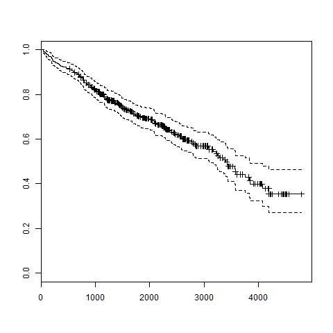
上图中的趋势有助于我们预测在特定天数结束时的生存概率。
R - Chi Square Test
Chi-Square test是一种统计方法,用于确定两个分类变量之间是否存在显着相关性。 这些变量都应来自同一群体,它们应该分类如:是/否,男/女,红/绿等。
例如,我们可以建立一个数据集,观察人们的冰淇淋购买模式,并尝试将人的性别与他们喜欢的冰淇淋的味道联系起来。 如果发现相关性,我们可以通过了解访问者的性别数量来计划适当的口味库存。
语法 (Syntax)
用于执行卡方检验的函数是chisq.test() 。
在R中创建卡方检验的基本语法是 -
chisq.test(data)
以下是所用参数的说明 -
data是表格形式的数据,包含观察中变量的计数值。
例子 (Example)
我们将在“MASS”库中获取Cars93数据,该库代表了1993年不同型号汽车的销售情况。
library("MASS")
print(str(Cars93))
当我们执行上面的代码时,它会产生以下结果 -
'data.frame': 93 obs. of 27 variables:
$ Manufacturer : Factor w/ 32 levels "Acura","Audi",..: 1 1 2 2 3 4 4 4 4 5 ...
$ Model : Factor w/ 93 levels "100","190E","240",..: 49 56 9 1 6 24 54 74 73 35 ...
$ Type : Factor w/ 6 levels "Compact","Large",..: 4 3 1 3 3 3 2 2 3 2 ...
$ Min.Price : num 12.9 29.2 25.9 30.8 23.7 14.2 19.9 22.6 26.3 33 ...
$ Price : num 15.9 33.9 29.1 37.7 30 15.7 20.8 23.7 26.3 34.7 ...
$ Max.Price : num 18.8 38.7 32.3 44.6 36.2 17.3 21.7 24.9 26.3 36.3 ...
$ MPG.city : int 25 18 20 19 22 22 19 16 19 16 ...
$ MPG.highway : int 31 25 26 26 30 31 28 25 27 25 ...
$ AirBags : Factor w/ 3 levels "Driver & Passenger",..: 3 1 2 1 2 2 2 2 2 2 ...
$ DriveTrain : Factor w/ 3 levels "4WD","Front",..: 2 2 2 2 3 2 2 3 2 2 ...
$ Cylinders : Factor w/ 6 levels "3","4","5","6",..: 2 4 4 4 2 2 4 4 4 5 ...
$ EngineSize : num 1.8 3.2 2.8 2.8 3.5 2.2 3.8 5.7 3.8 4.9 ...
$ Horsepower : int 140 200 172 172 208 110 170 180 170 200 ...
$ RPM : int 6300 5500 5500 5500 5700 5200 4800 4000 4800 4100 ...
$ Rev.per.mile : int 2890 2335 2280 2535 2545 2565 1570 1320 1690 1510 ...
$ Man.trans.avail : Factor w/ 2 levels "No","Yes": 2 2 2 2 2 1 1 1 1 1 ...
$ Fuel.tank.capacity: num 13.2 18 16.9 21.1 21.1 16.4 18 23 18.8 18 ...
$ Passengers : int 5 5 5 6 4 6 6 6 5 6 ...
$ Length : int 177 195 180 193 186 189 200 216 198 206 ...
$ Wheelbase : int 102 115 102 106 109 105 111 116 108 114 ...
$ Width : int 68 71 67 70 69 69 74 78 73 73 ...
$ Turn.circle : int 37 38 37 37 39 41 42 45 41 43 ...
$ Rear.seat.room : num 26.5 30 28 31 27 28 30.5 30.5 26.5 35 ...
$ Luggage.room : int 11 15 14 17 13 16 17 21 14 18 ...
$ Weight : int 2705 3560 3375 3405 3640 2880 3470 4105 3495 3620 ...
$ Origin : Factor w/ 2 levels "USA","non-USA": 2 2 2 2 2 1 1 1 1 1 ...
$ Make : Factor w/ 93 levels "Acura Integra",..: 1 2 4 3 5 6 7 9 8 10 ...
上述结果显示数据集具有许多因子变量,可以将其视为分类变量。 对于我们的模型,我们将考虑变量“AirBags”和“Type”。 在这里,我们的目的是找出所售汽车类型与其所拥有的气囊类型之间的任何显着相关性。 如果观察到相关性,我们可以估计哪种类型的汽车能够更好地销售哪种类型的气囊。
# Load the library.
library("MASS")
# Create a data frame from the main data set.
car.data <- data.frame(Cars93$AirBags, Cars93$Type)
# Create a table with the needed variables.
car.data = table(Cars93$AirBags, Cars93$Type)
print(car.data)
# Perform the Chi-Square test.
print(chisq.test(car.data))
当我们执行上面的代码时,它会产生以下结果 -
Compact Large Midsize Small Sporty Van
Driver & Passenger 2 4 7 0 3 0
Driver only 9 7 11 5 8 3
None 5 0 4 16 3 6
Pearson's Chi-squared test
data: car.data
X-squared = 33.001, df = 10, p-value = 0.0002723
Warning message:
In chisq.test(car.data) : Chi-squared approximation may be incorrect
结论 (Conclusion)
结果显示p值小于0.05,表明字符串相关。
