SciPy - ODR
ODR代表Orthogonal Distance Regression ,用于回归研究。 基本线性回归通常用于通过绘制图表上的最佳拟合线来估计两个变量y和x之间的关系。
用于此的数学方法称为Least Squares ,旨在最小化每个点的平方误差之和。 这里的关键问题是如何计算每个点的误差(也称为残差)?
在标准线性回归中,目标是从X值预测Y值 - 因此明智的做法是计算Y值中的误差(如下图中的灰线所示)。 但是,有时考虑X和Y中的误差更为明智(如下图中红色虚线所示)。
例如 - 当您知道X的测量值不确定时,或者您不想关注一个变量的误差而不是另一个变量的误差时。
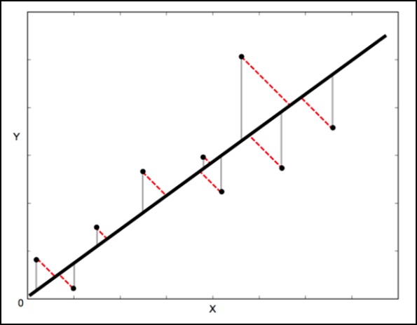
正交距离回归(ODR)是一种可以做到这一点的方法(在这种情况下正交意味着垂直 - 所以它计算垂直于线的误差,而不仅仅是'垂直')。
scipy.odr单变量回归的实现
以下示例演示了单变量回归的scipy.odr实现。
import numpy as np
import matplotlib.pyplot as plt
from scipy.odr import *
import random
# Initiate some data, giving some randomness using random.random().
x = np.array([0, 1, 2, 3, 4, 5])
y = np.array([i**2 + random.random() for i in x])
# Define a function (quadratic in our case) to fit the data with.
def linear_func(p, x):
   m, c = p
   return m*x + c
# Create a model for fitting.
linear_model = Model(linear_func)
# Create a RealData object using our initiated data from above.
data = RealData(x, y)
# Set up ODR with the model and data.
odr = ODR(data, linear_model, beta0=[0., 1.])
# Run the regression.
out = odr.run()
# Use the in-built pprint method to give us results.
out.pprint()
上述程序将生成以下输出。
Beta: [ 5.51846098 -4.25744878]
Beta Std Error: [ 0.7786442 2.33126407]
Beta Covariance: [
   [ 1.93150969 -4.82877433]
   [ -4.82877433 17.31417201
]]
Residual Variance: 0.313892697582
Inverse Condition #: 0.146618499389
Reason(s) for Halting:
   Sum of squares convergence
