R - 二项分布( Binomial Distribution)
二项分布模型用于找出事件成功的概率,该事件在一系列实验中仅具有两种可能的结果。 例如,投掷硬币总是给出头部或尾部。 在二项分布期间估计在重复投掷硬币10次时准确找到3个头的概率。
R有四个内置函数来生成二项分布。 它们如下所述。
dbinom(x, size, prob)
pbinom(x, size, prob)
qbinom(p, size, prob)
rbinom(n, size, prob)
以下是所用参数的说明 -
x是数字的向量。
p是概率的向量。
n是观察次数。
size是试验次数。
prob是每次试验成功的概率。
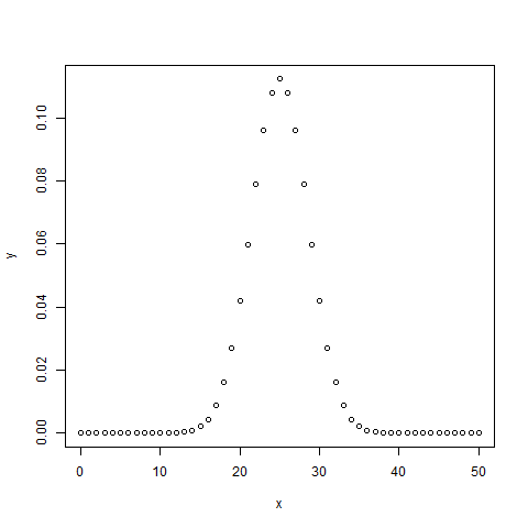
dbinom()
该函数给出了每个点的概率密度分布。
# Create a sample of 50 numbers which are incremented by 1.
x <- seq(0,50,by = 1)
# Create the binomial distribution.
y <- dbinom(x,50,0.5)
# Give the chart file a name.
png(file = "dbinom.png")
# Plot the graph for this sample.
plot(x,y)
# Save the file.
dev.off()
当我们执行上面的代码时,它会产生以下结果 -
pbinom()
此函数给出事件的累积概率。 它是表示概率的单个值。
# Probability of getting 26 or less heads from a 51 tosses of a coin.
x <- pbinom(26,51,0.5)
print(x)
当我们执行上面的代码时,它会产生以下结果 -
[1] 0.610116
qbinom()
此函数获取概率值并给出其累积值与概率值匹配的数字。
# How many heads will have a probability of 0.25 will come out when a coin
# is tossed 51 times.
x <- qbinom(0.25,51,1/2)
print(x)
当我们执行上面的代码时,它会产生以下结果 -
[1] 23
rbinom()
此函数从给定样本生成给定概率的所需数量的随机值。
# Find 8 random values from a sample of 150 with probability of 0.4.
x <- rbinom(8,150,.4)
print(x)
当我们执行上面的代码时,它会产生以下结果 -
[1] 58 61 59 66 55 60 61 67
