Python Pandas - 快速指南
Python Pandas - Introduction
Pandas是一个开源Python库,使用其强大的数据结构提供高性能数据操作和分析工具。 Pandas这个名字源自Panel Data - 来自多维数据的计量经济学。
2008年,开发人员Wes McKinney在需要高性能,灵活的数据分析工具时开始开发大熊猫。
在Pandas之前,Python主要用于数据整理和准备。 它对数据分析的贡献很小。 熊猫解决了这个问题。 使用Pandas,我们可以完成数据处理和分析中的五个典型步骤,无论数据来源如何 - 加载,准备,操作,建模和分析。
Python with Pandas用于广泛的领域,包括学术和商业领域,包括金融,经济,统计,分析等。
熊猫的主要特点
- 具有默认和自定义索引的快速高效的DataFrame对象。
- 用于将数据加载到来自不同文件格式的内存数据对象的工具。
- 数据对齐和缺失数据的集成处理。
- 日期集的重塑和旋转。
- 基于标签的切片,索引和大数据集的子集化。
- 可以删除或插入数据结构中的列。
- 按数据分组以进行聚合和转换。
- 高性能的合并和数据连接。
- 时间序列功能。
Python Pandas - Environment Setup
标准Python发行版不与Pandas模块捆绑在一起。 一个轻量级的替代方案是使用流行的Python包安装程序pip.安装NumPy pip.
pip install pandas
如果您安装Anaconda Python软件包,默认情况下将安装Pandas以下内容 -
Windows
Anaconda (来自https://www.continuum.io )是SciPy堆栈的免费Python发行版。 它也适用于Linux和Mac。
Canopy ( https://www.enthought.com/products/canopy/ )免费提供商业发行版,并提供适用于Windows,Linux和Mac的完整SciPy堆栈。
Python (x,y)是一个免费的Python发行版,包含SciPy堆栈和适用于Windows操作系统的Spyder IDE。 (可从http://python-xy.github.io/下载)
Linux
各个Linux发行版的软件包管理器用于在SciPy堆栈中安装一个或多个软件包。
For Ubuntu Users
sudo apt-get install python-numpy python-scipy python-matplotlibipythonipythonnotebook
python-pandas python-sympy python-nose
For Fedora Users
sudo yum install numpyscipy python-matplotlibipython python-pandas sympy
python-nose atlas-devel
Introduction to Data Structures
熊猫处理以下三种数据结构 -
- Series
- DataFrame
- Panel
这些数据结构构建在Numpy数组之上,这意味着它们很快。
尺寸和描述
考虑这些数据结构的最佳方式是较高维度的数据结构是其较低维度数据结构的容器。 例如,DataFrame是Series的容器,Panel是DataFrame的容器。
| 数据结构 | 外形尺寸 | 描述 |
|---|---|---|
| Series | 1 | 1D标记的同质阵列,sizeimmutable。 |
| 数据框架 | 2 | 一般2D标记的,尺寸可变的表格结构,具有潜在的异质类型柱。 |
| Panel | 3 | 一般3D标记,大小可变阵列。 |
构建和处理两个或更多维数组是一项繁琐的任务,在编写函数时,用户需要考虑数据集的方向。 但是使用Pandas数据结构,可以减少用户的心理努力。
例如,对于表格数据(DataFrame),考虑index (行)和columns而不是轴0和轴1在语义上更有帮助。
可变性(Mutability)
所有Pandas数据结构都是值可变的(可以更改),而Series Series都是大小可变的。 系列大小不可变。
Note - DataFrame被广泛使用,是最重要的数据结构之一。 面板的使用要少得多。
系列
系列是具有同质数据的一维数组结构。 例如,以下系列是整数10,23,56,...的集合。
| 10 | 23 | 56 | 17 | 52 | 61 | 73 | 90 | 26 | 72 |
关键点
- 同质数据
- Size Immutable
- 数据可变的值
DataFrame
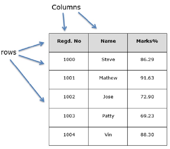
DataFrame是具有异构数据的二维数组。 例如,
| 名称 | 年龄 | 性别 | 评分 |
|---|---|---|---|
| Steve | 32 | Male | 3.45 |
| Lia | 28 | Female | 4.6 |
| Vin | 45 | Male | 3.9 |
| Katie | 38 | Female | 2.78 |
该表格表示组织销售团队的整体绩效评级数据。 数据以行和列表示。 每列代表一个属性,每行代表一个人。
列的数据类型
四列的数据类型如下 -
| 柱 | 类型 |
|---|---|
| Name | String |
| Age | Integer |
| Gender | String |
| Rating | Float |
关键点
- 异构数据
- 大小可变
- 数据可变
Panel
Panel是具有异构数据的三维数据结构。 很难用图形表示来表示面板。 但是可以将面板说明为DataFrame的容器。
关键点
- 异构数据
- 大小可变
- 数据可变
Python Pandas - Series
Series是一维标记数组,能够保存任何类型的数据(整数,字符串,浮点数,python对象等)。 轴标签统称为索引。
pandas.Series
可以使用以下构造函数创建pandas系列 -
pandas.Series( data, index, dtype, copy)
构造函数的参数如下 -
| S.No | 参数和描述 |
|---|---|
| 1 | data 数据采用各种形式,如ndarray,list,常量 |
| 2 | index 索引值必须是唯一且可清除的,与数据长度相同。 如果没有传递索引,则默认为np.arrange(n) 。 |
| 3 | dtype dtype用于数据类型。 如果为None,则将推断数据类型 |
| 4 | copy 复制数据。 默认为False |
可以使用各种输入创建系列,例如 -
- Array
- Dict
- Scalar value or constant
创建一个空系列
可以创建的基本系列是空系列。
例子 (Example)
#import the pandas library and aliasing as pd
import pandas as pd
s = pd.Series()
print s
其output如下 -
Series([], dtype: float64)
从ndarray创建一个系列
如果数据是ndarray,则传递的索引必须具有相同的长度。 如果没有传递索引,那么默认索引将是range(n) ,其中n是数组长度,即[0,1,2,3 .... range(len(array))-1].
例子1 (Example 1)
#import the pandas library and aliasing as pd
import pandas as pd
import numpy as np
data = np.array(['a','b','c','d'])
s = pd.Series(data)
print s
其output如下 -
0   a
1   b
2   c
3   d
dtype: object
我们没有传递任何索引,因此默认情况下,它分配的索引范围从0到len(data)-1 ,即0到3。
例子2 (Example 2)
#import the pandas library and aliasing as pd
import pandas as pd
import numpy as np
data = np.array(['a','b','c','d'])
s = pd.Series(data,index=[100,101,102,103])
print s
其output如下 -
100  a
101  b
102  c
103  d
dtype: object
我们在这里传递了索引值。 现在我们可以在输出中看到自定义的索引值。
从dict创建一个系列
可以将dict作为输入传递,如果未指定索引,则按排序顺序获取字典键以构造索引。 如果传递了索引,则将拉出与索引中的标签对应的数据中的值。
例子1 (Example 1)
#import the pandas library and aliasing as pd
import pandas as pd
import numpy as np
data = {'a' : 0., 'b' : 1., 'c' : 2.}
s = pd.Series(data)
print s
其output如下 -
a 0.0
b 1.0
c 2.0
dtype: float64
Observe - 字典键用于构造索引。
例子2 (Example 2)
#import the pandas library and aliasing as pd
import pandas as pd
import numpy as np
data = {'a' : 0., 'b' : 1., 'c' : 2.}
s = pd.Series(data,index=['b','c','d','a'])
print s
其output如下 -
b 1.0
c 2.0
d NaN
a 0.0
dtype: float64
Observe - 索引顺序是持久的,缺少的元素用NaN(非数字)填充。
从标量创建一个系列
如果数据是标量值,则必须提供索引。 将重复该值以匹配index的长度
#import the pandas library and aliasing as pd
import pandas as pd
import numpy as np
s = pd.Series(5, index=[0, 1, 2, 3])
print s
其output如下 -
0  5
1  5
2  5
3  5
dtype: int64
从具有位置的系列访问数据
系列中的数据可以类似于ndarray.中的数据访问ndarray.
例子1 (Example 1)
检索第一个元素。 我们已经知道,对于数组,计数从零开始,这意味着第一个元素存储在第零个位置,依此类推。
import pandas as pd
s = pd.Series([1,2,3,4,5],index = ['a','b','c','d','e'])
#retrieve the first element
print s[0]
其output如下 -
1
例子2 (Example 2)
检索系列中的前三个元素。 如果在其前面插入:,则将提取该索引以后的所有项目。 如果使用两个参数(在它们之间):两个索引之间的项目(不包括停止索引)
import pandas as pd
s = pd.Series([1,2,3,4,5],index = ['a','b','c','d','e'])
#retrieve the first three element
print s[:3]
其output如下 -
a  1
b  2
c  3
dtype: int64
例子3 (Example 3)
检索最后三个元素。
import pandas as pd
s = pd.Series([1,2,3,4,5],index = ['a','b','c','d','e'])
#retrieve the last three element
print s[-3:]
其output如下 -
c  3
d  4
e  5
dtype: int64
使用标签(索引)检索数据
Series类似于固定大小的dict ,您可以通过索引标签获取和设置值。
例子1 (Example 1)
使用索引标签值检索单个元素。
import pandas as pd
s = pd.Series([1,2,3,4,5],index = ['a','b','c','d','e'])
#retrieve a single element
print s['a']
其output如下 -
1
例子2 (Example 2)
使用索引标签值列表检索多个元素。
import pandas as pd
s = pd.Series([1,2,3,4,5],index = ['a','b','c','d','e'])
#retrieve multiple elements
print s[['a','c','d']]
其output如下 -
a  1
c  3
d  4
dtype: int64
例子3 (Example 3)
如果未包含标签,则会引发异常。
import pandas as pd
s = pd.Series([1,2,3,4,5],index = ['a','b','c','d','e'])
#retrieve multiple elements
print s['f']
其output如下 -
…
KeyError: 'f'
Python Pandas - DataFrame
数据框是二维数据结构,即数据以行和列的表格形式对齐。
DataFrame的功能
- 潜在的列有不同的类型
- 大小 - 可变
- 标记轴(行和列)
- 可以对行和列执行算术运算
结构 Structure
我们假设我们正在创建一个包含学生数据的数据框。
您可以将其视为SQL表或电子表格数据表示。
pandas.DataFrame
可以使用以下构造函数创建pandas DataFrame -
pandas.DataFrame( data, index, columns, dtype, copy)
构造函数的参数如下 -
| S.No | 参数和描述 |
|---|---|
| 1 | data 数据采用各种形式,如ndarray,系列,地图,列表,字典,常量以及另一个DataFrame。 |
| 2 | index 对于行标签,如果没有传递索引,则用于结果帧的索引是Optional Default np.arrange(n)。 |
| 3 | columns 对于列标签,可选的默认语法是 - np.arrange(n)。 仅当没有传递索引时才会出现这种情况。 |
| 4 | dtype 每列的数据类型。 |
| 4 | copy 如果默认值为False,则此命令(或其他任何命令)用于复制数据。 |
创建DataFrame
可以使用各种输入创建pandas DataFrame,例如 -
- Lists
- dict
- Series
- Numpy ndarrays
- 另一个DataFrame
在本章的后续部分中,我们将了解如何使用这些输入创建DataFrame。
创建一个空DataFrame
可以创建的基本DataFrame是空数据帧。
例子 (Example)
#import the pandas library and aliasing as pd
import pandas as pd
df = pd.DataFrame()
print df
其output如下 -
Empty DataFrame
Columns: []
Index: []
从列表中创建DataFrame
可以使用单个列表或列表列表创建DataFrame。
例子1 (Example 1)
import pandas as pd
data = [1,2,3,4,5]
df = pd.DataFrame(data)
print df
其output如下 -
     0
0    1
1    2
2    3
3    4
4    5
例子2 (Example 2)
import pandas as pd
data = [['Alex',10],['Bob',12],['Clarke',13]]
df = pd.DataFrame(data,columns=['Name','Age'])
print df
其output如下 -
      Name      Age
0     Alex      10
1     Bob       12
2     Clarke    13
例子3 (Example 3)
import pandas as pd
data = [['Alex',10],['Bob',12],['Clarke',13]]
df = pd.DataFrame(data,columns=['Name','Age'],dtype=float)
print df
其output如下 -
      Name     Age
0     Alex     10.0
1     Bob      12.0
2     Clarke   13.0
Note - 观察, dtype参数将Age列的类型更改为浮点。
从ndarrays/Lists的Dict创建一个DataFrame
所有的ndarrays必须具有相同的长度。 如果传递了index,那么索引的长度应该等于数组的长度。
如果没有传递索引,那么默认情况下,index将是range(n),其中n是数组长度。
例子1 (Example 1)
import pandas as pd
data = {'Name':['Tom', 'Jack', 'Steve', 'Ricky'],'Age':[28,34,29,42]}
df = pd.DataFrame(data)
print df
其output如下 -
      Age      Name
0     28        Tom
1     34       Jack
2     29      Steve
3     42      Ricky
Note - 观察值0,1,2,3。 它们是使用函数范围(n)分配给每个索引的默认索引。
例子2 (Example 2)
现在让我们使用数组创建一个索引的DataFrame。
import pandas as pd
data = {'Name':['Tom', 'Jack', 'Steve', 'Ricky'],'Age':[28,34,29,42]}
df = pd.DataFrame(data, index=['rank1','rank2','rank3','rank4'])
print df
其output如下 -
         Age    Name
rank1    28      Tom
rank2    34     Jack
rank3    29    Steve
rank4    42    Ricky
Note - 观察, index参数为每一行分配一个索引。
从Dicts列表创建一个DataFrame
字典列表可以作为输入数据传递以创建DataFrame。 默认情况下,字典键被视为列名。
例子1 (Example 1)
以下示例显示如何通过传递字典列表来创建DataFrame。
import pandas as pd
data = [{'a': 1, 'b': 2},{'a': 5, 'b': 10, 'c': 20}]
df = pd.DataFrame(data)
print df
其output如下 -
    a    b      c
0   1   2     NaN
1   5   10   20.0
Note - 观察,NaN(非数字)附加在缺失区域中。
例子2 (Example 2)
以下示例显示如何通过传递字典列表和行索引来创建DataFrame。
import pandas as pd
data = [{'a': 1, 'b': 2},{'a': 5, 'b': 10, 'c': 20}]
df = pd.DataFrame(data, index=['first', 'second'])
print df
其output如下 -
        a   b       c
first   1   2     NaN
second  5   10   20.0
例子3 (Example 3)
以下示例显示如何使用字典列表,行索引和列索引创建DataFrame。
import pandas as pd
data = [{'a': 1, 'b': 2},{'a': 5, 'b': 10, 'c': 20}]
#With two column indices, values same as dictionary keys
df1 = pd.DataFrame(data, index=['first', 'second'], columns=['a', 'b'])
#With two column indices with one index with other name
df2 = pd.DataFrame(data, index=['first', 'second'], columns=['a', 'b1'])
print df1
print df2
其output如下 -
#df1 output
         a  b
first    1  2
second   5  10
#df2 output
         a  b1
first    1  NaN
second   5  NaN
Note - 观察,df2使用除字典键以外的列索引创建DataFrame; 因此,将NaN附加到位。 而df1是使用与字典键相同的列索引创建的,因此附加了NaN。
从Dict of Series创建一个DataFrame
可以传递系列字典以形成DataFrame。 结果索引是传递的所有系列索引的并集。
例子 (Example)
import pandas as pd
d = {'one' : pd.Series([1, 2, 3], index=['a', 'b', 'c']),
      'two' : pd.Series([1, 2, 3, 4], index=['a', 'b', 'c', 'd'])}
df = pd.DataFrame(d)
print df
其output如下 -
      one    two
a     1.0    1
b     2.0    2
c     3.0    3
d     NaN    4
Note - 观察,对于系列1,没有传递标签'd' ,但在结果中,对于d标签,NaN附加了NaN。
现在让我们通过示例了解column selection, addition和deletion 。
列选择
我们将通过从DataFrame中选择一列来理解这一点。
例子 (Example)
import pandas as pd
d = {'one' : pd.Series([1, 2, 3], index=['a', 'b', 'c']),
      'two' : pd.Series([1, 2, 3, 4], index=['a', 'b', 'c', 'd'])}
df = pd.DataFrame(d)
print df ['one']
其output如下 -
a     1.0
b     2.0
c     3.0
d     NaN
Name: one, dtype: float64
列添加
我们将通过向现有数据框添加新列来理解这一点。
例子 (Example)
import pandas as pd
d = {'one' : pd.Series([1, 2, 3], index=['a', 'b', 'c']),
      'two' : pd.Series([1, 2, 3, 4], index=['a', 'b', 'c', 'd'])}
df = pd.DataFrame(d)
# Adding a new column to an existing DataFrame object with column label by passing new series
print ("Adding a new column by passing as Series:")
df['three']=pd.Series([10,20,30],index=['a','b','c'])
print df
print ("Adding a new column using the existing columns in DataFrame:")
df['four']=df['one']+df['three']
print df
其output如下 -
Adding a new column by passing as Series:
     one   two   three
a    1.0    1    10.0
b    2.0    2    20.0
c    3.0    3    30.0
d    NaN    4    NaN
Adding a new column using the existing columns in DataFrame:
      one   two   three    four
a     1.0    1    10.0     11.0
b     2.0    2    20.0     22.0
c     3.0    3    30.0     33.0
d     NaN    4     NaN     NaN
列删除
列可以删除或弹出; 让我们举一个例子来了解如何。
例子 (Example)
# Using the previous DataFrame, we will delete a column
# using del function
import pandas as pd
d = {'one' : pd.Series([1, 2, 3], index=['a', 'b', 'c']),
     'two' : pd.Series([1, 2, 3, 4], index=['a', 'b', 'c', 'd']),
     'three' : pd.Series([10,20,30], index=['a','b','c'])}
df = pd.DataFrame(d)
print ("Our dataframe is:")
print df
# using del function
print ("Deleting the first column using DEL function:")
del df['one']
print df
# using pop function
print ("Deleting another column using POP function:")
df.pop('two')
print df
其output如下 -
Our dataframe is:
      one   three  two
a     1.0    10.0   1
b     2.0    20.0   2
c     3.0    30.0   3
d     NaN     NaN   4
Deleting the first column using DEL function:
      three    two
a     10.0     1
b     20.0     2
c     30.0     3
d     NaN      4
Deleting another column using POP function:
   three
a  10.0
b  20.0
c  30.0
d  NaN
行选择,添加和删除
我们现在将通过示例了解行选择,添加和删除。 让我们从选择的概念开始。
按标签选择
可以通过将行标签传递给loc函数来选择行。import pandas as pd
d = {'one' : pd.Series([1, 2, 3], index=['a', 'b', 'c']),
'two' : pd.Series([1, 2, 3, 4], index=['a', 'b', 'c', 'd'])}
df = pd.DataFrame(d)
print df.loc['b']
其output如下 -
one 2.0
two 2.0
Name: b, dtype: float64
结果是一系列标签作为DataFrame的列名。 并且,系列的名称是用于检索它的标签。
按整数位置选择
可以通过将整数位置传递给iloc函数来选择行。
import pandas as pd
d = {'one' : pd.Series([1, 2, 3], index=['a', 'b', 'c']),
     'two' : pd.Series([1, 2, 3, 4], index=['a', 'b', 'c', 'd'])}
df = pd.DataFrame(d)
print df.iloc[2]
其output如下 -
one   3.0
two   3.0
Name: c, dtype: float64
切片行
可以使用':'运算符选择多行。
import pandas as pd
d = {'one' : pd.Series([1, 2, 3], index=['a', 'b', 'c']),
    'two' : pd.Series([1, 2, 3, 4], index=['a', 'b', 'c', 'd'])}
df = pd.DataFrame(d)
print df[2:4]
其output如下 -
      one    two
c     3.0     3
d     NaN     4
添加行
使用append函数向DataFrame添加新行。 此函数将在末尾附加行。
import pandas as pd
df = pd.DataFrame([[1, 2], [3, 4]], columns = ['a','b'])
df2 = pd.DataFrame([[5, 6], [7, 8]], columns = ['a','b'])
df = df.append(df2)
print df
其output如下 -
   a  b
0  1  2
1  3  4
0  5  6
1  7  8
删除行
使用索引标签从DataFrame中删除或删除行。 如果标签重复,则将删除多行。
如果您观察到,在上面的示例中,标签是重复的。 让我们删除一个标签,看看会丢弃多少行。
import pandas as pd
df = pd.DataFrame([[1, 2], [3, 4]], columns = ['a','b'])
df2 = pd.DataFrame([[5, 6], [7, 8]], columns = ['a','b'])
df = df.append(df2)
# Drop rows with label 0
df = df.drop(0)
print df
其output如下 -
  a b
1 3 4
1 7 8
在上面的示例中,删除了两行,因为这两行包含相同的标签0。
Python Pandas - Panel
panel是数据的3D容器。 术语Panel data来源于计量经济学,并且部分负责名称pandas - pan(el)-da(ta) -s。
3轴的名称旨在为描述涉及面板数据的操作提供一些语义含义。 他们是 -
items - axis 0,每个项目对应一个包含在其中的DataFrame。
major_axis - 轴1,它是每个DataFrame的索引(行)。
minor_axis - 轴2,它是每个DataFrame的列。
pandas.Panel()
可以使用以下构造函数创建Panel -
pandas.Panel(data, items, major_axis, minor_axis, dtype, copy)
构造函数的参数如下 -
| 参数 | 描述 |
|---|---|
| data | 数据采用各种形式,如ndarray,系列,地图,列表,字典,常量以及另一个DataFrame |
| items | axis=0 |
| major_axis | axis=1 |
| minor_axis | axis=2 |
| dtype | 每列的数据类型 |
| copy | 复制数据。 默认, false |
创建面板
可以使用多种方式创建Panel,例如 -
- 来自ndarrays
- 来自DataFrames的dict
来自3D ndarray
# creating an empty panel
import pandas as pd
import numpy as np
data = np.random.rand(2,4,5)
p = pd.Panel(data)
print p
其output如下 -
<class 'pandas.core.panel.Panel'>
Dimensions: 2 (items) x 4 (major_axis) x 5 (minor_axis)
Items axis: 0 to 1
Major_axis axis: 0 to 3
Minor_axis axis: 0 to 4
Note - 观察空面板和上面板的尺寸,所有对象都不同。
来自DataFrame Objects的dict
#creating an empty panel
import pandas as pd
import numpy as np
data = {'Item1' : pd.DataFrame(np.random.randn(4, 3)),
        'Item2' : pd.DataFrame(np.random.randn(4, 2))}
p = pd.Panel(data)
print p
其output如下 -
<class 'pandas.core.panel.Panel'>
Dimensions: 2 (items) x 4 (major_axis) x 5 (minor_axis)
Items axis: 0 to 1
Major_axis axis: 0 to 3
Minor_axis axis: 0 to 4
创建一个空面板
可以使用Panel构造函数创建一个空面板,如下所示 -
#creating an empty panel
import pandas as pd
p = pd.Panel()
print p
其output如下 -
<class 'pandas.core.panel.Panel'>
Dimensions: 0 (items) x 0 (major_axis) x 0 (minor_axis)
Items axis: None
Major_axis axis: None
Minor_axis axis: None
从面板中选择数据
使用 - 从面板中选择数据 -
- Items
- Major_axis
- Minor_axis
使用物品
# creating an empty panel
import pandas as pd
import numpy as np
data = {'Item1' : pd.DataFrame(np.random.randn(4, 3)),
        'Item2' : pd.DataFrame(np.random.randn(4, 2))}
p = pd.Panel(data)
print p['Item1']
其output如下 -
            0          1          2
0    0.488224  -0.128637   0.930817
1    0.417497   0.896681   0.576657
2   -2.775266   0.571668   0.290082
3   -0.400538  -0.144234   1.110535
我们有两个项目,我们检索了item1。 结果是一个包含4行和3列的Major_axis ,它们是Major_axis和Minor_axis维度。
使用major_axis
可以使用方法panel.major_axis(index)访问数据。
# creating an empty panel
import pandas as pd
import numpy as np
data = {'Item1' : pd.DataFrame(np.random.randn(4, 3)),
        'Item2' : pd.DataFrame(np.random.randn(4, 2))}
p = pd.Panel(data)
print p.major_xs(1)
其output如下 -
      Item1       Item2
0   0.417497    0.748412
1   0.896681   -0.557322
2   0.576657       NaN
使用minor_axis
可以使用方法panel.minor_axis(index).访问数据panel.minor_axis(index).
# creating an empty panel
import pandas as pd
import numpy as np
data = {'Item1' : pd.DataFrame(np.random.randn(4, 3)),
        'Item2' : pd.DataFrame(np.random.randn(4, 2))}
p = pd.Panel(data)
print p.minor_xs(1)
其output如下 -
       Item1       Item2
0   -0.128637   -1.047032
1    0.896681   -0.557322
2    0.571668    0.431953
3   -0.144234    1.302466
Note - 观察尺寸的变化。
Python Pandas - Basic Functionality
到目前为止,我们了解了三个Pandas DataStructures以及如何创建它们。 我们将主要关注DataFrame对象,因为它在实时数据处理中很重要,并且还讨论了一些其他DataStructures。
系列基本功能
| S.No. | 属性或方法 | 描述 |
|---|---|---|
| 1 | axes | 返回行轴标签的列表。 |
| 2 | dtype | 返回对象的dtype。 |
| 3 | empty | 如果系列为空,则返回True。 |
| 4 | ndim | 根据定义1,返回基础数据的维数。 |
| 5 | size | 返回基础数据中的元素数。 |
| 6 | values | 将系列返回为ndarray。 |
| 7 | head() | 返回前n行。 |
| 8 | tail() | 返回最后n行。 |
现在让我们创建一个Series并查看上面列出的所有属性操作。
例子 (Example)
import pandas as pd
import numpy as np
#Create a series with 100 random numbers
s = pd.Series(np.random.randn(4))
print s
其output如下 -
0   0.967853
1  -0.148368
2  -1.395906
3  -1.758394
dtype: float64
axes
返回系列标签的列表。
import pandas as pd
import numpy as np
#Create a series with 100 random numbers
s = pd.Series(np.random.randn(4))
print ("The axes are:")
print s.axes
其output如下 -
The axes are:
[RangeIndex(start=0, stop=4, step=1)]
上述结果是从0到5的值列表的紧凑格式,即[0,1,2,3,4]。
empty
返回表示Object是否为空的布尔值。 True表示对象为空。
import pandas as pd
import numpy as np
#Create a series with 100 random numbers
s = pd.Series(np.random.randn(4))
print ("Is the Object empty?")
print s.empty
其output如下 -
Is the Object empty?
False
ndim
返回对象的维数。 根据定义,Series是一维数据结构,因此它返回
import pandas as pd
import numpy as np
#Create a series with 4 random numbers
s = pd.Series(np.random.randn(4))
print s
print ("The dimensions of the object:")
print s.ndim
其output如下 -
0   0.175898
1   0.166197
2  -0.609712
3  -1.377000
dtype: float64
The dimensions of the object:
1
尺寸
返回系列的大小(长度)。
import pandas as pd
import numpy as np
#Create a series with 4 random numbers
s = pd.Series(np.random.randn(2))
print s
print ("The size of the object:")
print s.size
其output如下 -
0   3.078058
1  -1.207803
dtype: float64
The size of the object:
2
values
以数组形式返回系列中的实际数据。
import pandas as pd
import numpy as np
#Create a series with 4 random numbers
s = pd.Series(np.random.randn(4))
print s
print ("The actual data series is:")
print s.values
其output如下 -
0   1.787373
1  -0.605159
2   0.180477
3  -0.140922
dtype: float64
The actual data series is:
[ 1.78737302 -0.60515881 0.18047664 -0.1409218 ]
头和尾
要查看Series或DataFrame对象的小样本,请使用head()和tail()方法。
head()返回前n行(观察索引值)。 要显示的默认元素数为5,但您可以传递自定义数字。
import pandas as pd
import numpy as np
#Create a series with 4 random numbers
s = pd.Series(np.random.randn(4))
print ("The original series is:")
print s
print ("The first two rows of the data series:")
print s.head(2)
其output如下 -
The original series is:
0   0.720876
1  -0.765898
2   0.479221
3  -0.139547
dtype: float64
The first two rows of the data series:
0   0.720876
1  -0.765898
dtype: float64
tail()返回最后n行(观察索引值)。 要显示的默认元素数为5,但您可以传递自定义数字。
import pandas as pd
import numpy as np
#Create a series with 4 random numbers
s = pd.Series(np.random.randn(4))
print ("The original series is:")
print s
print ("The last two rows of the data series:")
print s.tail(2)
其output如下 -
The original series is:
0 -0.655091
1 -0.881407
2 -0.608592
3 -2.341413
dtype: float64
The last two rows of the data series:
2 -0.608592
3 -2.341413
dtype: float64
DataFrame基本功能
现在让我们了解DataFrame基本功能是什么。 下表列出了有助于DataFrame基本功能的重要属性或方法。
| S.No. | 属性或方法 | 描述 |
|---|---|---|
| 1 | T | 转置行和列。 |
| 2 | axes | 返回一个列表,其中行轴标签和列轴标签为唯一成员。 |
| 3 | dtypes | 返回此对象中的dtypes。 |
| 4 | empty | 如果NDFrame完全为空,则为True [无项目]; 如果任何轴的长度为0。 |
| 5 | ndim | 轴数/数组尺寸。 |
| 6 | shape | 返回表示DataFrame维度的元组。 |
| 7 | size | NDFrame中的元素数。 |
| 8 | values | NDFrame的Numpy表示。 |
| 9 | head() | 返回前n行。 |
| 10 | tail() | 返回最后n行。 |
现在让我们创建一个DataFrame,并查看上述属性的运行方式。
例子 (Example)
import pandas as pd
import numpy as np
#Create a Dictionary of series
d = {'Name':pd.Series(['Tom','James','Ricky','Vin','Steve','Smith','Jack']),
   'Age':pd.Series([25,26,25,23,30,29,23]),
   'Rating':pd.Series([4.23,3.24,3.98,2.56,3.20,4.6,3.8])}
#Create a DataFrame
df = pd.DataFrame(d)
print ("Our data series is:")
print df
其output如下 -
Our data series is:
    Age   Name    Rating
0   25    Tom     4.23
1   26    James   3.24
2   25    Ricky   3.98
3   23    Vin     2.56
4   30    Steve   3.20
5   29    Smith   4.60
6   23    Jack    3.80
T (Transpose)
返回DataFrame的转置。 行和列将互换。
import pandas as pd
import numpy as np
# Create a Dictionary of series
d = {'Name':pd.Series(['Tom','James','Ricky','Vin','Steve','Smith','Jack']),
   'Age':pd.Series([25,26,25,23,30,29,23]),
   'Rating':pd.Series([4.23,3.24,3.98,2.56,3.20,4.6,3.8])}
# Create a DataFrame
df = pd.DataFrame(d)
print ("The transpose of the data series is:")
print df.T
其output如下 -
The transpose of the data series is:
         0     1       2      3      4      5       6
Age      25    26      25     23     30     29      23
Name     Tom   James   Ricky  Vin    Steve  Smith   Jack
Rating   4.23  3.24    3.98   2.56   3.2    4.6     3.8
axes
返回行轴标签和列轴标签的列表。
import pandas as pd
import numpy as np
#Create a Dictionary of series
d = {'Name':pd.Series(['Tom','James','Ricky','Vin','Steve','Smith','Jack']),
   'Age':pd.Series([25,26,25,23,30,29,23]),
   'Rating':pd.Series([4.23,3.24,3.98,2.56,3.20,4.6,3.8])}
#Create a DataFrame
df = pd.DataFrame(d)
print ("Row axis labels and column axis labels are:")
print df.axes
其output如下 -
Row axis labels and column axis labels are:
[RangeIndex(start=0, stop=7, step=1), Index([u'Age', u'Name', u'Rating'],
dtype='object')]
dtypes
返回每列的数据类型。
import pandas as pd
import numpy as np
#Create a Dictionary of series
d = {'Name':pd.Series(['Tom','James','Ricky','Vin','Steve','Smith','Jack']),
   'Age':pd.Series([25,26,25,23,30,29,23]),
   'Rating':pd.Series([4.23,3.24,3.98,2.56,3.20,4.6,3.8])}
#Create a DataFrame
df = pd.DataFrame(d)
print ("The data types of each column are:")
print df.dtypes
其output如下 -
The data types of each column are:
Age     int64
Name    object
Rating  float64
dtype: object
empty
返回表示Object是否为空的布尔值; True表示对象为空。
import pandas as pd
import numpy as np
#Create a Dictionary of series
d = {'Name':pd.Series(['Tom','James','Ricky','Vin','Steve','Smith','Jack']),
   'Age':pd.Series([25,26,25,23,30,29,23]),
   'Rating':pd.Series([4.23,3.24,3.98,2.56,3.20,4.6,3.8])}
#Create a DataFrame
df = pd.DataFrame(d)
print ("Is the object empty?")
print df.empty
其output如下 -
Is the object empty?
False
ndim
返回对象的维数。 根据定义,DataFrame是一个2D对象。
import pandas as pd
import numpy as np
#Create a Dictionary of series
d = {'Name':pd.Series(['Tom','James','Ricky','Vin','Steve','Smith','Jack']),
   'Age':pd.Series([25,26,25,23,30,29,23]),
   'Rating':pd.Series([4.23,3.24,3.98,2.56,3.20,4.6,3.8])}
#Create a DataFrame
df = pd.DataFrame(d)
print ("Our object is:")
print df
print ("The dimension of the object is:")
print df.ndim
其output如下 -
Our object is:
      Age    Name     Rating
0     25     Tom      4.23
1     26     James    3.24
2     25     Ricky    3.98
3     23     Vin      2.56
4     30     Steve    3.20
5     29     Smith    4.60
6     23     Jack     3.80
The dimension of the object is:
2
shape
返回表示DataFrame维度的元组。 元组(a,b),其中a表示行数, b表示列数。
import pandas as pd
import numpy as np
#Create a Dictionary of series
d = {'Name':pd.Series(['Tom','James','Ricky','Vin','Steve','Smith','Jack']),
   'Age':pd.Series([25,26,25,23,30,29,23]),
   'Rating':pd.Series([4.23,3.24,3.98,2.56,3.20,4.6,3.8])}
#Create a DataFrame
df = pd.DataFrame(d)
print ("Our object is:")
print df
print ("The shape of the object is:")
print df.shape
其output如下 -
Our object is:
   Age   Name    Rating
0  25    Tom     4.23
1  26    James   3.24
2  25    Ricky   3.98
3  23    Vin     2.56
4  30    Steve   3.20
5  29    Smith   4.60
6  23    Jack    3.80
The shape of the object is:
(7, 3)
尺寸
返回DataFrame中的元素数。
import pandas as pd
import numpy as np
#Create a Dictionary of series
d = {'Name':pd.Series(['Tom','James','Ricky','Vin','Steve','Smith','Jack']),
   'Age':pd.Series([25,26,25,23,30,29,23]),
   'Rating':pd.Series([4.23,3.24,3.98,2.56,3.20,4.6,3.8])}
#Create a DataFrame
df = pd.DataFrame(d)
print ("Our object is:")
print df
print ("The total number of elements in our object is:")
print df.size
其output如下 -
Our object is:
    Age   Name    Rating
0   25    Tom     4.23
1   26    James   3.24
2   25    Ricky   3.98
3   23    Vin     2.56
4   30    Steve   3.20
5   29    Smith   4.60
6   23    Jack    3.80
The total number of elements in our object is:
21
values
将数据框中的实际数据作为NDarray.
import pandas as pd
import numpy as np
#Create a Dictionary of series
d = {'Name':pd.Series(['Tom','James','Ricky','Vin','Steve','Smith','Jack']),
   'Age':pd.Series([25,26,25,23,30,29,23]),
   'Rating':pd.Series([4.23,3.24,3.98,2.56,3.20,4.6,3.8])}
#Create a DataFrame
df = pd.DataFrame(d)
print ("Our object is:")
print df
print ("The actual data in our data frame is:")
print df.values
其output如下 -
Our object is:
    Age   Name    Rating
0   25    Tom     4.23
1   26    James   3.24
2   25    Ricky   3.98
3   23    Vin     2.56
4   30    Steve   3.20
5   29    Smith   4.60
6   23    Jack    3.80
The actual data in our data frame is:
[[25 'Tom' 4.23]
[26 'James' 3.24]
[25 'Ricky' 3.98]
[23 'Vin' 2.56]
[30 'Steve' 3.2]
[29 'Smith' 4.6]
[23 'Jack' 3.8]]
头和尾
要查看DataFrame对象的一小部分示例,请使用head()和tail()方法。 head()返回前n行(观察索引值)。 要显示的默认元素数为5,但您可以传递自定义数字。
import pandas as pd
import numpy as np
#Create a Dictionary of series
d = {'Name':pd.Series(['Tom','James','Ricky','Vin','Steve','Smith','Jack']),
   'Age':pd.Series([25,26,25,23,30,29,23]),
   'Rating':pd.Series([4.23,3.24,3.98,2.56,3.20,4.6,3.8])}
#Create a DataFrame
df = pd.DataFrame(d)
print ("Our data frame is:")
print df
print ("The first two rows of the data frame is:")
print df.head(2)
其output如下 -
Our data frame is:
    Age   Name    Rating
0   25    Tom     4.23
1   26    James   3.24
2   25    Ricky   3.98
3   23    Vin     2.56
4   30    Steve   3.20
5   29    Smith   4.60
6   23    Jack    3.80
The first two rows of the data frame is:
   Age   Name   Rating
0  25    Tom    4.23
1  26    James  3.24
tail()返回最后n行(观察索引值)。 要显示的默认元素数为5,但您可以传递自定义数字。
import pandas as pd
import numpy as np
#Create a Dictionary of series
d = {'Name':pd.Series(['Tom','James','Ricky','Vin','Steve','Smith','Jack']),
   'Age':pd.Series([25,26,25,23,30,29,23]),
   'Rating':pd.Series([4.23,3.24,3.98,2.56,3.20,4.6,3.8])}
#Create a DataFrame
df = pd.DataFrame(d)
print ("Our data frame is:")
print df
print ("The last two rows of the data frame is:")
print df.tail(2)
其output如下 -
Our data frame is:
    Age   Name    Rating
0   25    Tom     4.23
1   26    James   3.24
2   25    Ricky   3.98
3   23    Vin     2.56
4   30    Steve   3.20
5   29    Smith   4.60
6   23    Jack    3.80
The last two rows of the data frame is:
    Age   Name    Rating
5   29    Smith    4.6
6   23    Jack     3.8
Python Pandas - Descriptive Statistics
大量方法共同计算DataFrame上的描述性统计和其他相关操作。 其中大多数是sum(), mean(),等聚合sum(), mean(),但其中一些(如sumsum()生成相同大小的对象。 一般来说,这些方法采用axis参数,就像ndarray.{sum, std, ...},但轴可以通过名称或整数指定
DataFrame - “index”(axis = 0,默认值),“columns”(axis = 1)
让我们创建一个DataFrame,并在本章的所有操作中使用此对象。
例子 (Example)
import pandas as pd
import numpy as np
#Create a Dictionary of series
d = {'Name':pd.Series(['Tom','James','Ricky','Vin','Steve','Smith','Jack',
   'Lee','David','Gasper','Betina','Andres']),
   'Age':pd.Series([25,26,25,23,30,29,23,34,40,30,51,46]),
   'Rating':pd.Series([4.23,3.24,3.98,2.56,3.20,4.6,3.8,3.78,2.98,4.80,4.10,3.65])}
#Create a DataFrame
df = pd.DataFrame(d)
print df
其output如下 -
    Age  Name   Rating
0   25   Tom     4.23
1   26   James   3.24
2   25   Ricky   3.98
3   23   Vin     2.56
4   30   Steve   3.20
5   29   Smith   4.60
6   23   Jack    3.80
7   34   Lee     3.78
8   40   David   2.98
9   30   Gasper  4.80
10  51   Betina  4.10
11  46   Andres  3.65
sum()
返回请求轴的值的总和。 默认情况下,axis是index(axis = 0)。
import pandas as pd
import numpy as np
#Create a Dictionary of series
d = {'Name':pd.Series(['Tom','James','Ricky','Vin','Steve','Smith','Jack',
   'Lee','David','Gasper','Betina','Andres']),
   'Age':pd.Series([25,26,25,23,30,29,23,34,40,30,51,46]),
   'Rating':pd.Series([4.23,3.24,3.98,2.56,3.20,4.6,3.8,3.78,2.98,4.80,4.10,3.65])}
#Create a DataFrame
df = pd.DataFrame(d)
print df.sum()
其output如下 -
Age                                                    382
Name     TomJamesRickyVinSteveSmithJackLeeDavidGasperBe...
Rating                                               44.92
dtype: object
每个单独的列都单独添加(附加字符串)。
axis=1
此语法将提供如下所示的输出。
import pandas as pd
import numpy as np
#Create a Dictionary of series
d = {'Name':pd.Series(['Tom','James','Ricky','Vin','Steve','Smith','Jack',
   'Lee','David','Gasper','Betina','Andres']),
   'Age':pd.Series([25,26,25,23,30,29,23,34,40,30,51,46]),
   'Rating':pd.Series([4.23,3.24,3.98,2.56,3.20,4.6,3.8,3.78,2.98,4.80,4.10,3.65])}
#Create a DataFrame
df = pd.DataFrame(d)
print df.sum(1)
其output如下 -
0    29.23
1    29.24
2    28.98
3    25.56
4    33.20
5    33.60
6    26.80
7    37.78
8    42.98
9    34.80
10   55.10
11   49.65
dtype: float64
mean()
返回平均值
import pandas as pd
import numpy as np
#Create a Dictionary of series
d = {'Name':pd.Series(['Tom','James','Ricky','Vin','Steve','Smith','Jack',
   'Lee','David','Gasper','Betina','Andres']),
   'Age':pd.Series([25,26,25,23,30,29,23,34,40,30,51,46]),
   'Rating':pd.Series([4.23,3.24,3.98,2.56,3.20,4.6,3.8,3.78,2.98,4.80,4.10,3.65])}
#Create a DataFrame
df = pd.DataFrame(d)
print df.mean()
其output如下 -
Age       31.833333
Rating     3.743333
dtype: float64
std()
返回数值列的Bressel标准偏差。
import pandas as pd
import numpy as np
#Create a Dictionary of series
d = {'Name':pd.Series(['Tom','James','Ricky','Vin','Steve','Smith','Jack',
   'Lee','David','Gasper','Betina','Andres']),
   'Age':pd.Series([25,26,25,23,30,29,23,34,40,30,51,46]),
   'Rating':pd.Series([4.23,3.24,3.98,2.56,3.20,4.6,3.8,3.78,2.98,4.80,4.10,3.65])}
#Create a DataFrame
df = pd.DataFrame(d)
print df.std()
其output如下 -
Age       9.232682
Rating    0.661628
dtype: float64
功能和描述
现在让我们了解Python Pandas中描述性统计下的函数。 下表列出了重要的功能 -
| S.No. | 功能 | 描述 |
|---|---|---|
| 1 | count() | 非空观察的数量 |
| 2 | sum() | 价值总和 |
| 3 | mean() | 价值观的平均值 |
| 4 | median() | 价值中心 |
| 5 | mode() | 价值观 |
| 6 | std() | 标准值的偏差 |
| 7 | min() | 最低价值 |
| 8 | max() | 最大价值 |
| 9 | abs() | 绝对值 |
| 10 | prod() | 价值的产物 |
| 11 | cumsum() | 累积总和 |
| 12 | cumprod() | 累积产品 |
Note - 由于DataFrame是异构数据结构。 通用操作不适用于所有功能。
sum(), cumsum()等函数可以使用数字和字符(或)字符串数据元素,而不会出现任何错误。 虽然n练习,但通常不会使用字符聚合,这些函数不会抛出任何异常。
当datFrame包含字符或字符串数据时abs(), cumprod()等函数会抛出异常,因为无法执行此类操作。
总结数据
describe()函数计算与DataFrame列有关的统计信息摘要。
import pandas as pd
import numpy as np
#Create a Dictionary of series
d = {'Name':pd.Series(['Tom','James','Ricky','Vin','Steve','Smith','Jack',
   'Lee','David','Gasper','Betina','Andres']),
   'Age':pd.Series([25,26,25,23,30,29,23,34,40,30,51,46]),
   'Rating':pd.Series([4.23,3.24,3.98,2.56,3.20,4.6,3.8,3.78,2.98,4.80,4.10,3.65])}
#Create a DataFrame
df = pd.DataFrame(d)
print df.describe()
其output如下 -
               Age         Rating
count    12.000000      12.000000
mean     31.833333       3.743333
std       9.232682       0.661628
min      23.000000       2.560000
25%      25.000000       3.230000
50%      29.500000       3.790000
75%      35.500000       4.132500
max      51.000000       4.800000
此函数提供mean, std和IQR值。 并且,函数排除了有关数字列的字符列和给定的摘要。 'include'是用于传递有关哪些列需要考虑用于汇总的必要信息的参数。 获取值列表; 默认情况下,'数字'。
- object - 汇总String列
- number - 汇总数字列
- all - 将所有列汇总在一起(不应将其作为列表值传递)
现在,在程序中使用以下语句并检查输出 -
import pandas as pd
import numpy as np
#Create a Dictionary of series
d = {'Name':pd.Series(['Tom','James','Ricky','Vin','Steve','Smith','Jack',
   'Lee','David','Gasper','Betina','Andres']),
   'Age':pd.Series([25,26,25,23,30,29,23,34,40,30,51,46]),
   'Rating':pd.Series([4.23,3.24,3.98,2.56,3.20,4.6,3.8,3.78,2.98,4.80,4.10,3.65])}
#Create a DataFrame
df = pd.DataFrame(d)
print df.describe(include=['object'])
其output如下 -
          Name
count       12
unique      12
top      Ricky
freq         1
现在,使用以下语句并检查输出 -
import pandas as pd
import numpy as np
#Create a Dictionary of series
d = {'Name':pd.Series(['Tom','James','Ricky','Vin','Steve','Smith','Jack',
   'Lee','David','Gasper','Betina','Andres']),
   'Age':pd.Series([25,26,25,23,30,29,23,34,40,30,51,46]),
   'Rating':pd.Series([4.23,3.24,3.98,2.56,3.20,4.6,3.8,3.78,2.98,4.80,4.10,3.65])}
#Create a DataFrame
df = pd.DataFrame(d)
print df. describe(include='all')
其output如下 -
          Age          Name       Rating
count   12.000000        12    12.000000
unique        NaN        12          NaN
top           NaN     Ricky          NaN
freq          NaN         1          NaN
mean    31.833333       NaN     3.743333
std      9.232682       NaN     0.661628
min     23.000000       NaN     2.560000
25%     25.000000       NaN     3.230000
50%     29.500000       NaN     3.790000
75%     35.500000       NaN     4.132500
max     51.000000       NaN     4.800000
Python Pandas - Function Application
要将您自己或其他库的函数应用于Pandas对象,您应该了解三个重要方法。 这些方法已在下面讨论。 使用的适当方法取决于您的函数是期望在整个DataFrame,行或列方式还是元素方式上运行。
- 表明功能应用:管道()
- 行或列智能函数应用程序:apply()
- 元素智能函数应用程序:applymap()
逐表函数应用
可以通过将函数和适当数量的参数作为管道参数传递来执行自定义操作。 因此,对整个DataFrame执行操作。
例如,为DataFrame中的所有元素添加值2。 然后,
加法器功能
加法器函数添加两个数值作为参数并返回总和。
def adder(ele1,ele2):
return ele1+ele2
我们现在将使用自定义函数对DataFrame进行操作。
df = pd.DataFrame(np.random.randn(5,3),columns=['col1','col2','col3'])
df.pipe(adder,2)
让我们看看完整的节目 -
import pandas as pd
import numpy as np
def adder(ele1,ele2):
   return ele1+ele2
df = pd.DataFrame(np.random.randn(5,3),columns=['col1','col2','col3'])
df.pipe(adder,2)
print df.apply(np.mean)
其output如下 -
        col1       col2       col3
0   2.176704   2.219691   1.509360
1   2.222378   2.422167   3.953921
2   2.241096   1.135424   2.696432
3   2.355763   0.376672   1.182570
4   2.308743   2.714767   2.130288
行或列智能函数应用程序
可以使用apply()方法沿DataFrame或Panel的轴应用任意函数,该方法与描述性统计方法一样,采用可选的轴参数。 默认情况下,操作按列方式执行,将每列作为类似数组。
例子1 (Example 1)
import pandas as pd
import numpy as np
df = pd.DataFrame(np.random.randn(5,3),columns=['col1','col2','col3'])
df.apply(np.mean)
print df.apply(np.mean)
其output如下 -
      col1       col2        col3
0   0.343569  -1.013287    1.131245
1   0.508922  -0.949778   -1.600569
2  -1.182331  -0.420703   -1.725400
3   0.860265   2.069038   -0.537648
4   0.876758  -0.238051    0.473992
通过传递axis参数,可以逐行执行操作。
例子2 (Example 2)
import pandas as pd
import numpy as np
df = pd.DataFrame(np.random.randn(5,3),columns=['col1','col2','col3'])
df.apply(np.mean,axis=1)
print df.apply(np.mean)
其output如下 -
     col1         col2         col3
0  0.543255    -1.613418    -0.500731
1  0.976543    -1.135835    -0.719153
2  0.184282    -0.721153    -2.876206
3  0.447738     0.268062    -1.937888
4 -0.677673     0.177455     1.397360
例子3 (Example 3)
import pandas as pd
import numpy as np
df = pd.DataFrame(np.random.randn(5,3),columns=['col1','col2','col3'])
df.apply(lambda x: x.max() - x.min())
print df.apply(np.mean)
其output如下 -
       col1        col2      col3
0   -0.585206   -0.104938   1.424115
1   -0.326036   -1.444798   0.196849
2   -2.033478    1.682253   1.223152
3   -0.107015    0.499846   0.084127
4   -1.046964   -1.935617  -0.009919
元素智能函数应用
并非所有函数都可以进行矢量化(NumPy数组既不返回另一个数组也不是任何值), applymap()上的方法applymap()和analogously map()系列上的analogously map()接受任何采用单个值并返回单个值的Python函数。
例子1 (Example 1)
import pandas as pd
import numpy as np
df = pd.DataFrame(np.random.randn(5,3),columns=['col1','col2','col3'])
# My custom function
df['col1'].map(lambda x:x*100)
print df.apply(np.mean)
其output如下 -
<pre class="result notranslate">       col1      col2       col3
0    0.629348  0.088467  -1.790702
1   -0.592595  0.184113  -1.524998
2   -0.419298  0.262369  -0.178849
3   -1.036930  1.103169   0.941882
4   -0.573333 -0.031056   0.315590
</pre>
例子2 (Example 2)
import pandas as pd
import numpy as np
# My custom function
df = pd.DataFrame(np.random.randn(5,3),columns=['col1','col2','col3'])
df.applymap(lambda x:x*100)
print df.apply(np.mean)
其output如下 -
output is as follows:
         col1         col2         col3
0   17.670426    21.969052    -49.064031
1   22.237846    42.216693     195.392124
2   24.109576   -86.457646     69.643171
3   35.576312   -162.332803   -81.743023
4   30.874333    71.476717     13.028751
Python Pandas - Reindexing
Reindexing更改DataFrame的行标签和列标签。 重新索引意味着使数据符合以匹配特定轴上的给定标签集。
可以通过索引来完成多个操作,如 -
重新排序现有数据以匹配一组新标签。
在标签位置插入缺失值(NA)标记,其中不存在标签数据。
例子 (Example)
import pandas as pd
import numpy as np
N=20
df = pd.DataFrame({
   'A': pd.date_range(start='2016-01-01',periods=N,freq='D'),
   'x': np.linspace(0,stop=N-1,num=N),
   'y': np.random.rand(N),
   'C': np.random.choice(['Low','Medium','High'],N).tolist(),
   'D': np.random.normal(100, 10, size=(N)).tolist()
})
#reindex the DataFrame
df_reindexed = df.reindex(index=[0,2,5], columns=['A', 'C', 'B'])
print df_reindexed
其output如下 -
            A    C     B
0  2016-01-01  Low   NaN
2  2016-01-03  High  NaN
5  2016-01-06  Low   NaN
重新索引以与其他对象对齐
您可能希望获取一个对象并重新索引其轴标记与另一个对象相同。 请考虑以下示例以了解相同的情况。
例子 (Example)
import pandas as pd
import numpy as np
df1 = pd.DataFrame(np.random.randn(10,3),columns=['col1','col2','col3'])
df2 = pd.DataFrame(np.random.randn(7,3),columns=['col1','col2','col3'])
df1 = df1.reindex_like(df2)
print df1
其output如下 -
          col1         col2         col3
0    -2.467652    -1.211687    -0.391761
1    -0.287396     0.522350     0.562512
2    -0.255409    -0.483250     1.866258
3    -1.150467    -0.646493    -0.222462
4     0.152768    -2.056643     1.877233
5    -1.155997     1.528719    -1.343719
6    -1.015606    -1.245936    -0.295275
Note - 这里, df1 DataFrame被改变并重新编制索引,如df2 。 列名称应匹配,否则将为整个列标签添加NAN。
重新索引时填充
reindex()接受一个可选的参数方法,这是一个填充方法,其值如下 -
pad/ffill - 向前填充值
bfill/backfill - 向后填充值
nearest - 从最近的索引值填写
例子 (Example)
import pandas as pd
import numpy as np
df1 = pd.DataFrame(np.random.randn(6,3),columns=['col1','col2','col3'])
df2 = pd.DataFrame(np.random.randn(2,3),columns=['col1','col2','col3'])
# Padding NAN's
print df2.reindex_like(df1)
# Now Fill the NAN's with preceding Values
print ("Data Frame with Forward Fill:")
print df2.reindex_like(df1,method='ffill')
其output如下 -
         col1        col2       col3
0    1.311620   -0.707176   0.599863
1   -0.423455   -0.700265   1.133371
2         NaN         NaN        NaN
3         NaN         NaN        NaN
4         NaN         NaN        NaN
5         NaN         NaN        NaN
Data Frame with Forward Fill:
         col1        col2        col3
0    1.311620   -0.707176    0.599863
1   -0.423455   -0.700265    1.133371
2   -0.423455   -0.700265    1.133371
3   -0.423455   -0.700265    1.133371
4   -0.423455   -0.700265    1.133371
5   -0.423455   -0.700265    1.133371
Note - 最后四行是填充的。
重新索引时填充的限制
limit参数在重建索引时提供对填充的额外控制。 限制指定连续匹配的最大数量。 让我们考虑下面的例子来理解相同的 -
例子 (Example)
import pandas as pd
import numpy as np
df1 = pd.DataFrame(np.random.randn(6,3),columns=['col1','col2','col3'])
df2 = pd.DataFrame(np.random.randn(2,3),columns=['col1','col2','col3'])
# Padding NAN's
print df2.reindex_like(df1)
# Now Fill the NAN's with preceding Values
print ("Data Frame with Forward Fill limiting to 1:")
print df2.reindex_like(df1,method='ffill',limit=1)
其output如下 -
         col1        col2        col3
0    0.247784    2.128727    0.702576
1   -0.055713   -0.021732   -0.174577
2         NaN         NaN         NaN
3         NaN         NaN         NaN
4         NaN         NaN         NaN
5         NaN         NaN         NaN
Data Frame with Forward Fill limiting to 1:
         col1        col2        col3
0    0.247784    2.128727    0.702576
1   -0.055713   -0.021732   -0.174577
2   -0.055713   -0.021732   -0.174577
3         NaN         NaN         NaN
4         NaN         NaN         NaN
5         NaN         NaN         NaN
Note - 观察,只有第7行由前面的第6行填充。 然后,按原样保留行。
Renaming
rename()方法允许您根据某些映射(字典或系列)或任意函数重新标记轴。
让我们考虑以下示例来理解这一点 -
import pandas as pd
import numpy as np
df1 = pd.DataFrame(np.random.randn(6,3),columns=['col1','col2','col3'])
print df1
print ("After renaming the rows and columns:")
print df1.rename(columns={'col1' : 'c1', 'col2' : 'c2'},
index = {0 : 'apple', 1 : 'banana', 2 : 'durian'})
其output如下 -
         col1        col2        col3
0    0.486791    0.105759    1.540122
1   -0.990237    1.007885   -0.217896
2   -0.483855   -1.645027   -1.194113
3   -0.122316    0.566277   -0.366028
4   -0.231524   -0.721172   -0.112007
5    0.438810    0.000225    0.435479
After renaming the rows and columns:
                c1          c2        col3
apple     0.486791    0.105759    1.540122
banana   -0.990237    1.007885   -0.217896
durian   -0.483855   -1.645027   -1.194113
3        -0.122316    0.566277   -0.366028
4        -0.231524   -0.721172   -0.112007
5         0.438810    0.000225    0.435479
rename()方法提供了一个inplace命名参数,默认情况下为False并复制基础数据。 inplace=True以重命名数据。
Python Pandas - Iteration
基于Pandas对象的基本迭代行为取决于类型。 迭代一系列时,它被视为类似数组,基本迭代产生值。 其他数据结构,如DataFrame和Panel,遵循迭代对象keys的dict-like约定。
简而言之,基本迭代(对象中的i )产生 -
Series - 价值观
DataFrame - 列标签
Panel - 项目标签
迭代DataFrame
迭代DataFrame会给出列名。 让我们考虑以下示例来理解相同的内容。
import pandas as pd
import numpy as np
N=20
df = pd.DataFrame({
    'A': pd.date_range(start='2016-01-01',periods=N,freq='D'),
    'x': np.linspace(0,stop=N-1,num=N),
    'y': np.random.rand(N),
    'C': np.random.choice(['Low','Medium','High'],N).tolist(),
    'D': np.random.normal(100, 10, size=(N)).tolist()
    })
for col in df:
   print col
其output如下 -
A
C
D
x
y
要迭代DataFrame的行,我们可以使用以下函数 -
iteritems() - 迭代(键,值)对
iterrows() - 迭代行(索引,系列)对
itertuples() - 作为itertuples()迭代行
iteritems()
迭代每列作为键,值对,标签为键,列值为Series对象。
import pandas as pd
import numpy as np
df = pd.DataFrame(np.random.randn(4,3),columns = ['col1','col2','col3'])
for key,value in df.iteritems():
   print key,value
其output如下 -
col1 0    0.802390
1    0.324060
2    0.256811
3    0.839186
Name: col1, dtype: float64
col2 0    1.624313
1   -1.033582
2    1.796663
3    1.856277
Name: col2, dtype: float64
col3 0   -0.022142
1   -0.230820
2    1.160691
3   -0.830279
Name: col3, dtype: float64
观察,每列作为系列中的键值对单独迭代。
iterrows()
iterrows()返回迭代器,产生每个索引值以及包含每行数据的系列。
import pandas as pd
import numpy as np
df=pd.DataFrame(np.random.randn(4,3),columns=['col1','col2','col3'])
for row_index,row in df.iterrows():
   print row_index,row
其output如下 -
0  col1    1.529759
   col2    0.762811
   col3   -0.634691
Name: 0, dtype: float64
1  col1   -0.944087
   col2    1.420919
   col3   -0.507895
Name: 1, dtype: float64
2  col1   -0.077287
   col2   -0.858556
   col3   -0.663385
Name: 2, dtype: float64
3  col1    -1.638578
   col2     0.059866
   col3     0.493482
Name: 3, dtype: float64
Note - 由于iterrows()遍历行,因此它不会保留整行的数据类型。 0,1,2是行索引,col1,col2,col3是列索引。
itertuples()
itertuples()方法将返回一个迭代器,为DataFrame中的每一行产生一个命名元组。 元组的第一个元素是行的相应索引值,而其余值是行值。
import pandas as pd
import numpy as np
df = pd.DataFrame(np.random.randn(4,3),columns = ['col1','col2','col3'])
for row in df.itertuples():
   print row
其output如下 -
Pandas(Index=0, col1=1.5297586201375899, col2=0.76281127433814944, col3=-
0.6346908238310438)
Pandas(Index=1, col1=-0.94408735763808649, col2=1.4209186418359423, col3=-
0.50789517967096232)
Pandas(Index=2, col1=-0.07728664756791935, col2=-0.85855574139699076, col3=-
0.6633852507207626)
Pandas(Index=3, col1=0.65734942534106289, col2=-0.95057710432604969,
col3=0.80344487462316527)
Note - 迭代时不要尝试修改任何对象。 迭代用于读取,迭代器返回原始对象(视图)的副本,因此更改不会反映在原始对象上。
import pandas as pd
import numpy as np
df = pd.DataFrame(np.random.randn(4,3),columns = ['col1','col2','col3'])
for index, row in df.iterrows():
   row['a'] = 10
print df
其output如下 -
        col1       col2       col3
0  -1.739815   0.735595  -0.295589
1   0.635485   0.106803   1.527922
2  -0.939064   0.547095   0.038585
3  -1.016509  -0.116580  -0.523158
观察,没有反映出变化。
Python Pandas - Sorting
Pandas中有两种排序方式。 他们是 -
- 按标签
- By Actual Value
让我们考虑一个带输出的例子。
import pandas as pd
import numpy as np
unsorted_df=pd.DataFrame(np.random.randn(10,2),index=[1,4,6,2,3,5,9,8,0,7],colu
mns=['col2','col1'])
print unsorted_df
其output如下 -
        col2       col1
1  -2.063177   0.537527
4   0.142932  -0.684884
6   0.012667  -0.389340
2  -0.548797   1.848743
3  -1.044160   0.837381
5   0.385605   1.300185
9   1.031425  -1.002967
8  -0.407374  -0.435142
0   2.237453  -1.067139
7  -1.445831  -1.701035
在unsorted_df , labels和values未排序。 让我们看看如何对它们进行排序。
按标签
使用sort_index()方法,通过传递轴参数和排序顺序,可以对DataFrame进行排序。 默认情况下,按行升序对行标签进行排序。
import pandas as pd
import numpy as np
unsorted_df = pd.DataFrame(np.random.randn(10,2),index=[1,4,6,2,3,5,9,8,0,7],colu
   mns = ['col2','col1'])
sorted_df=unsorted_df.sort_index()
print sorted_df
其output如下 -
        col2       col1
0   0.208464   0.627037
1   0.641004   0.331352
2  -0.038067  -0.464730
3  -0.638456  -0.021466
4   0.014646  -0.737438
5  -0.290761  -1.669827
6  -0.797303  -0.018737
7   0.525753   1.628921
8  -0.567031   0.775951
9   0.060724  -0.322425
排序顺序
通过将布尔值传递给升序参数,可以控制排序的顺序。 让我们考虑以下示例来理解相同的内容。
import pandas as pd
import numpy as np
unsorted_df = pd.DataFrame(np.random.randn(10,2),index=[1,4,6,2,3,5,9,8,0,7],colu
   mns = ['col2','col1'])
sorted_df = unsorted_df.sort_index(ascending=False)
print sorted_df
其output如下 -
         col2        col1
9    0.825697    0.374463
8   -1.699509    0.510373
7   -0.581378    0.622958
6   -0.202951    0.954300
5   -1.289321   -1.551250
4    1.302561    0.851385
3   -0.157915   -0.388659
2   -1.222295    0.166609
1    0.584890   -0.291048
0    0.668444   -0.061294
对列进行排序
通过将axis参数传递给值0或1,可以在列标签上完成排序。 默认情况下,axis = 0,按行排序。 让我们考虑以下示例来理解相同的内容。
import pandas as pd
import numpy as np
unsorted_df = pd.DataFrame(np.random.randn(10,2),index=[1,4,6,2,3,5,9,8,0,7],colu
   mns = ['col2','col1'])
sorted_df=unsorted_df.sort_index(axis=1)
print sorted_df
其output如下 -
         col1        col2
1   -0.291048    0.584890
4    0.851385    1.302561
6    0.954300   -0.202951
2    0.166609   -1.222295
3   -0.388659   -0.157915
5   -1.551250   -1.289321
9    0.374463    0.825697
8    0.510373   -1.699509
0   -0.061294    0.668444
7    0.622958   -0.581378
按价值
与索引排序一样, sort_values()是按值排序的方法。 它接受一个'by'参数,该参数将使用要对其值进行排序的DataFrame的列名。
import pandas as pd
import numpy as np
unsorted_df = pd.DataFrame({'col1':[2,1,1,1],'col2':[1,3,2,4]})
sorted_df = unsorted_df.sort_values(by='col1')
print sorted_df
其output如下 -
   col1  col2
1    1    3
2    1    2
3    1    4
0    2    1
观察,col1值被排序,相应的col2值和行索引将与col1一起改变。 因此,他们看起来没有分类。
'by'参数采用列值列表。
import pandas as pd
import numpy as np
unsorted_df = pd.DataFrame({'col1':[2,1,1,1],'col2':[1,3,2,4]})
   sorted_df = unsorted_df.sort_values(by=['col1','col2'])
print sorted_df
其output如下 -
  col1 col2
2   1   2
1   1   3
3   1   4
0   2   1
排序算法
sort_values()提供了从mergesort,heapsort和quicksort中选择算法的规定。 Mergesort是唯一稳定的算法。
import pandas as pd
import numpy as np
unsorted_df = pd.DataFrame({'col1':[2,1,1,1],'col2':[1,3,2,4]})
sorted_df = unsorted_df.sort_values(by='col1' ,kind='mergesort')
print sorted_df
其output如下 -
  col1 col2
1    1    3
2    1    2
3    1    4
0    2    1
Python Pandas - Working with Text Data
在本章中,我们将讨论基本系列/索引的字符串操作。 在随后的章节中,我们将学习如何在DataFrame上应用这些字符串函数。
Pandas提供了一组字符串函数,可以轻松地对字符串数据进行操作。 最重要的是,这些函数忽略(或排除)缺失/ NaN值。
几乎所有这些方法都适用于Python字符串函数(参见: https://docs.python.org/3/library/stdtypes.html#string-methods : https://docs.python.org/3/library/stdtypes.html#string-methods )。 因此,将Series Object转换为String Object,然后执行操作。
现在让我们看看每个操作的执行情况。
| S.No | 功能 | 描述 |
|---|---|---|
| 1 | lower() | 将Series/Index中的字符串转换为小写。 |
| 2 | upper() | 将Series/Index中的字符串转换为大写。 |
| 3 | len() | 计算字符串长度()。 |
| 4 | strip() | 帮助从两侧的系列/索引中的每个字符串中剥离空白(包括换行符)。 |
| 5 | 分裂(' ') | 使用给定模式拆分每个字符串。 |
| 6 | 猫(sep ='') | 使用给定的分隔符连接系列/索引元素。 |
| 7 | get_dummies() | 返回具有One-Hot编码值的DataFrame。 |
| 8 | contains(pattern) | 如果子元素包含在元素中,则返回每个元素的布尔值True,否则返回False。 |
| 9 | replace(a,b) | 用值b替换值b 。 |
| 10 | repeat(value) | 以指定的次数重复每个元素。 |
| 11 | count(pattern) | 返回每个元素中pattern的外观计数。 |
| 12 | startswith(pattern) | 如果Series/Index中的元素以模式开头,则返回true。 |
| 13 | endswith(pattern) | 如果Series/Index中的元素以模式结束,则返回true。 |
| 14 | find(pattern) | 返回第一次出现的模式的第一个位置。 |
| 15 | findall(pattern) | 返回所有模式的列表。 |
| 16 | swapcase | 将表壳置于下/上。 |
| 17 | islower() | 检查Series/Index中每个字符串中的所有字符是否均为小写。 返回布尔值 |
| 18 | isupper() | 检查Series/Index中每个字符串中的所有字符是否都是大写。 返回布尔值。 |
| 19 | isnumeric() | 检查Series/Index中每个字符串中的所有字符是否都是数字。 返回布尔值。 |
现在让我们创建一个系列,看看上述所有功能是如何工作的。
import pandas as pd
import numpy as np
s = pd.Series(['Tom', 'William Rick', 'John', 'Alber@t', np.nan, '1234','SteveSmith'])
print s
其output如下 -
0            Tom
1   William Rick
2           John
3        Alber@t
4            NaN
5           1234
6    Steve Smith
dtype: object
lower()
import pandas as pd
import numpy as np
s = pd.Series(['Tom', 'William Rick', 'John', 'Alber@t', np.nan, '1234','SteveSmith'])
print s.str.lower()
其output如下 -
0            tom
1   william rick
2           john
3        alber@t
4            NaN
5           1234
6    steve smith
dtype: object
upper()
import pandas as pd
import numpy as np
s = pd.Series(['Tom', 'William Rick', 'John', 'Alber@t', np.nan, '1234','SteveSmith'])
print s.str.upper()
其output如下 -
0            TOM
1   WILLIAM RICK
2           JOHN
3        ALBER@T
4            NaN
5           1234
6    STEVE SMITH
dtype: object
len()
import pandas as pd
import numpy as np
s = pd.Series(['Tom', 'William Rick', 'John', 'Alber@t', np.nan, '1234','SteveSmith'])
print s.str.len()
其output如下 -
0    3.0
1   12.0
2    4.0
3    7.0
4    NaN
5    4.0
6   10.0
dtype: float64
strip()
import pandas as pd
import numpy as np
s = pd.Series(['Tom ', ' William Rick', 'John', 'Alber@t'])
print s
print ("After Stripping:")
print s.str.strip()
其output如下 -
0            Tom
1   William Rick
2           John
3        Alber@t
dtype: object
After Stripping:
0            Tom
1   William Rick
2           John
3        Alber@t
dtype: object
split(pattern)
import pandas as pd
import numpy as np
s = pd.Series(['Tom ', ' William Rick', 'John', 'Alber@t'])
print s
print ("Split Pattern:")
print s.str.split(' ')
其output如下 -
0            Tom
1   William Rick
2           John
3        Alber@t
dtype: object
Split Pattern:
0   [Tom, , , , , , , , , , ]
1   [, , , , , William, Rick]
2   [John]
3   [Alber@t]
dtype: object
cat(sep=pattern)
import pandas as pd
import numpy as np
s = pd.Series(['Tom ', ' William Rick', 'John', 'Alber@t'])
print s.str.cat(sep='_')
其output如下 -
Tom _ William Rick_John_Alber@t
get_dummies()
import pandas as pd
import numpy as np
s = pd.Series(['Tom ', ' William Rick', 'John', 'Alber@t'])
print s.str.get_dummies()
其output如下 -
   William Rick   Alber@t   John   Tom
0             0         0      0     1
1             1         0      0     0
2             0         0      1     0
3             0         1      0     0
contains ()
import pandas as pd
s = pd.Series(['Tom ', ' William Rick', 'John', 'Alber@t'])
print s.str.contains(' ')
其output如下 -
0   True
1   True
2   False
3   False
dtype: bool
replace(a,b)
import pandas as pd
s = pd.Series(['Tom ', ' William Rick', 'John', 'Alber@t'])
print s
print ("After replacing @ with $:")
print s.str.replace('@','$')
其output如下 -
0   Tom
1   William Rick
2   John
3   Alber@t
dtype: object
After replacing @ with $:
0   Tom
1   William Rick
2   John
3   Alber$t
dtype: object
repeat(value)
import pandas as pd
s = pd.Series(['Tom ', ' William Rick', 'John', 'Alber@t'])
print s.str.repeat(2)
其output如下 -
0   Tom            Tom
1   William Rick   William Rick
2                  JohnJohn
3                  Alber@tAlber@t
dtype: object
count(pattern)
import pandas as pd
s = pd.Series(['Tom ', ' William Rick', 'John', 'Alber@t'])
print ("The number of 'm's in each string:")
print s.str.count('m')
其output如下 -
The number of 'm's in each string:
0    1
1    1
2    0
3    0
startswith(pattern)
import pandas as pd
s = pd.Series(['Tom ', ' William Rick', 'John', 'Alber@t'])
print ("Strings that start with 'T':")
print s.str. startswith ('T')
其output如下 -
0  True
1  False
2  False
3  False
dtype: bool
endswith(pattern)
import pandas as pd
s = pd.Series(['Tom ', ' William Rick', 'John', 'Alber@t'])
print ("Strings that end with 't':")
print s.str.endswith('t')
其output如下 -
Strings that end with 't':
0  False
1  False
2  False
3  True
dtype: bool
find(pattern)
import pandas as pd
s = pd.Series(['Tom ', ' William Rick', 'John', 'Alber@t'])
print s.str.find('e')
其output如下 -
0 -1
1 -1
2 -1
3 3
dtype: int64
“-1”表示元素中没有这样的模式。
findall(pattern)
import pandas as pd
s = pd.Series(['Tom ', ' William Rick', 'John', 'Alber@t'])
print s.str.findall('e')
其output如下 -
0 []
1 []
2 []
3 [e]
dtype: object
空列表([])表示元素中没有此类模式。
swapcase()
import pandas as pd
s = pd.Series(['Tom', 'William Rick', 'John', 'Alber@t'])
print s.str.swapcase()
其output如下 -
0 tOM
1 wILLIAM rICK
2 jOHN
3 aLBER@T
dtype: object
islower()
import pandas as pd
s = pd.Series(['Tom', 'William Rick', 'John', 'Alber@t'])
print s.str.islower()
其output如下 -
0 False
1 False
2 False
3 False
dtype: bool
isupper()
import pandas as pd
s = pd.Series(['Tom', 'William Rick', 'John', 'Alber@t'])
print s.str.isupper()
其output如下 -
0 False
1 False
2 False
3 False
dtype: bool
isnumeric()
import pandas as pd
s = pd.Series(['Tom', 'William Rick', 'John', 'Alber@t'])
print s.str.isnumeric()
其output如下 -
0 False
1 False
2 False
3 False
dtype: bool
Python Pandas - Options and Customization
Pandas提供API来定制其行为的某些方面,显示器主要使用。
API由五个相关功能组成。 他们是 -
- get_option()
- set_option()
- reset_option()
- describe_option()
- option_context()
现在让我们了解这些功能是如何运作的。
get_option(param)
get_option接受一个参数并返回下面输出中给出的值 -
display.max_rows
显示默认值。 解释器读取此值并显示具有此值的行作为显示的上限。
import pandas as pd
print pd.get_option("display.max_rows")
其output如下 -
60
display.max_columns
显示默认值。 解释器读取此值并显示具有此值的行作为显示的上限。
import pandas as pd
print pd.get_option("display.max_columns")
其output如下 -
20
这里,60和20是默认配置参数值。
set_option(param,value)
set_option接受两个参数并将值设置为参数,如下所示 -
display.max_rows
使用set_option() ,我们可以更改要显示的默认行数。
import pandas as pd
pd.set_option("display.max_rows",80)
print pd.get_option("display.max_rows")
其output如下 -
80
display.max_rows
使用set_option() ,我们可以更改要显示的默认行数。
import pandas as pd
pd.set_option("display.max_columns",30)
print pd.get_option("display.max_columns")
其output如下 -
30
reset_option(param)
reset_option接受一个参数并将值设置回默认值。
display.max_rows
使用reset_option(),我们可以将值更改回要显示的默认行数。
import pandas as pd
pd.reset_option("display.max_rows")
print pd.get_option("display.max_rows")
其output如下 -
60
describe_option(param)
describe_option打印参数的描述。
display.max_rows
使用reset_option(),我们可以将值更改回要显示的默认行数。
import pandas as pd
pd.describe_option("display.max_rows")
其output如下 -
display.max_rows : int
If max_rows is exceeded, switch to truncate view. Depending on
'large_repr', objects are either centrally truncated or printed as
a summary view. 'None' value means unlimited.
In case python/IPython is running in a terminal and `large_repr`
equals 'truncate' this can be set to 0 and pandas will auto-detect
the height of the terminal and print a truncated object which fits
the screen height. The IPython notebook, IPython qtconsole, or
IDLE do not run in a terminal and hence it is not possible to do
correct auto-detection.
[default: 60] [currently: 60]
option_context()
option_context上下文管理器用于临时设置with statement的选项。 退出with block时会自动恢复选项值 -
display.max_rows
使用option_context(),我们可以临时设置该值。
import pandas as pd
with pd.option_context("display.max_rows",10):
print(pd.get_option("display.max_rows"))
print(pd.get_option("display.max_rows"))
其output如下 -
10
10
请参阅第一个和第二个打印语句之间的区别。 第一个语句打印由option_context()设置的值,该值在with context本身中是临时的。 在with context ,第二个print语句打印配置的值。
经常使用的参数
| S.No | 参数 | 描述 |
|---|---|---|
| 1 | display.max_rows | 显示要显示的最大行数 |
| 2 | 2 display.max_columns | 显示要显示的最大列数 |
| 3 | display.expand_frame_repr | 将数据框显示为拉伸页面 |
| 4 | display.max_colwidth | 显示最大列宽 |
| 5 | display.precision | 显示十进制数的精度 |
Python Pandas - Indexing and Selecting Data
在本章中,我们将讨论如何对日期进行切片和切块,并且通常会获得pandas对象的子集。
Python和NumPy索引运算符“[]”和属性运算符“。” 可以在各种用例中快速轻松地访问Pandas数据结构。 但是,由于要访问的数据类型不是预先知道的,因此直接使用标准运算符会有一些优化限制。 对于生产代码,我们建议您利用本章中介绍的优化的pandas数据访问方法。
熊猫现在支持三种类型的多轴索引; 下表中提到了这三种类型 -
| 索引 | 描述 |
|---|---|
| .loc() | 基于标签 |
| .iloc() | 基于整数 |
| .ix() | 基于Label和Integer |
.loc()
Pandas提供了各种方法来进行纯粹label based indexing 。 切片时,还包括起始边界。 整数是有效标签,但它们是指标签而不是位置。
.loc()有多种访问方法,如 -
- 单个标量标签
- A list of labels
- A slice object
- 布尔数组
loc采用两个单独的/列表/范围运算符,用','分隔。 第一个表示行,第二个表示列。
例子1 (Example 1)
#import the pandas library and aliasing as pd
import pandas as pd
import numpy as np
df = pd.DataFrame(np.random.randn(8, 4),
index = ['a','b','c','d','e','f','g','h'], columns = ['A', 'B', 'C', 'D'])
#select all rows for a specific column
print df.loc[:,'A']
其output如下 -
a 0.391548
b -0.070649
c -0.317212
d -2.162406
e 2.202797
f 0.613709
g 1.050559
h 1.122680
Name: A, dtype: float64
例子2 (Example 2)
# import the pandas library and aliasing as pd
import pandas as pd
import numpy as np
df = pd.DataFrame(np.random.randn(8, 4),
index = ['a','b','c','d','e','f','g','h'], columns = ['A', 'B', 'C', 'D'])
# Select all rows for multiple columns, say list[]
print df.loc[:,['A','C']]
其output如下 -
A C
a 0.391548 0.745623
b -0.070649 1.620406
c -0.317212 1.448365
d -2.162406 -0.873557
e 2.202797 0.528067
f 0.613709 0.286414
g 1.050559 0.216526
h 1.122680 -1.621420
例子3 (Example 3)
# import the pandas library and aliasing as pd
import pandas as pd
import numpy as np
df = pd.DataFrame(np.random.randn(8, 4),
index = ['a','b','c','d','e','f','g','h'], columns = ['A', 'B', 'C', 'D'])
# Select few rows for multiple columns, say list[]
print df.loc[['a','b','f','h'],['A','C']]
其output如下 -
A C
a 0.391548 0.745623
b -0.070649 1.620406
f 0.613709 0.286414
h 1.122680 -1.621420
例子4 (Example 4)
# import the pandas library and aliasing as pd
import pandas as pd
import numpy as np
df = pd.DataFrame(np.random.randn(8, 4),
index = ['a','b','c','d','e','f','g','h'], columns = ['A', 'B', 'C', 'D'])
# Select range of rows for all columns
print df.loc['a':'h']
其output如下 -
A B C D
a 0.391548 -0.224297 0.745623 0.054301
b -0.070649 -0.880130 1.620406 1.419743
c -0.317212 -1.929698 1.448365 0.616899
d -2.162406 0.614256 -0.873557 1.093958
e 2.202797 -2.315915 0.528067 0.612482
f 0.613709 -0.157674 0.286414 -0.500517
g 1.050559 -2.272099 0.216526 0.928449
h 1.122680 0.324368 -1.621420 -0.741470
例子5 (Example 5)
# import the pandas library and aliasing as pd
import pandas as pd
import numpy as np
df = pd.DataFrame(np.random.randn(8, 4),
index = ['a','b','c','d','e','f','g','h'], columns = ['A', 'B', 'C', 'D'])
# for getting values with a boolean array
print df.loc['a']>0
其output如下 -
A False
B True
C False
D False
Name: a, dtype: bool
.iloc()
Pandas提供各种方法以获得纯粹基于整数的索引。 像python和numpy一样,这些都是0-based索引。
各种访问方法如下 -
- 一个整数
- A list of integers
- A range of values
例子1 (Example 1)
# import the pandas library and aliasing as pd
import pandas as pd
import numpy as np
df = pd.DataFrame(np.random.randn(8, 4), columns = ['A', 'B', 'C', 'D'])
# select all rows for a specific column
print df.iloc[:4]
其output如下 -
A B C D
0 0.699435 0.256239 -1.270702 -0.645195
1 -0.685354 0.890791 -0.813012 0.631615
2 -0.783192 -0.531378 0.025070 0.230806
3 0.539042 -1.284314 0.826977 -0.026251
例子2 (Example 2)
import pandas as pd
import numpy as np
df = pd.DataFrame(np.random.randn(8, 4), columns = ['A', 'B', 'C', 'D'])
# Integer slicing
print df.iloc[:4]
print df.iloc[1:5, 2:4]
其output如下 -
A B C D
0 0.699435 0.256239 -1.270702 -0.645195
1 -0.685354 0.890791 -0.813012 0.631615
2 -0.783192 -0.531378 0.025070 0.230806
3 0.539042 -1.284314 0.826977 -0.026251
C D
1 -0.813012 0.631615
2 0.025070 0.230806
3 0.826977 -0.026251
4 1.423332 1.130568
例子3 (Example 3)
import pandas as pd
import numpy as np
df = pd.DataFrame(np.random.randn(8, 4), columns = ['A', 'B', 'C', 'D'])
# Slicing through list of values
print df.iloc[[1, 3, 5], [1, 3]]
print df.iloc[1:3, :]
print df.iloc[:,1:3]
其output如下 -
B D
1 0.890791 0.631615
3 -1.284314 -0.026251
5 -0.512888 -0.518930
A B C D
1 -0.685354 0.890791 -0.813012 0.631615
2 -0.783192 -0.531378 0.025070 0.230806
B C
0 0.256239 -1.270702
1 0.890791 -0.813012
2 -0.531378 0.025070
3 -1.284314 0.826977
4 -0.460729 1.423332
5 -0.512888 0.581409
6 -1.204853 0.098060
7 -0.947857 0.641358
.ix()
除了基于纯标签和整数之外,Pandas还提供了一种混合方法,用于使用.ix()运算符对对象进行选择和子集化。
例子1 (Example 1)
import pandas as pd
import numpy as np
df = pd.DataFrame(np.random.randn(8, 4), columns = ['A', 'B', 'C', 'D'])
# Integer slicing
print df.ix[:4]
其output如下 -
A B C D
0 0.699435 0.256239 -1.270702 -0.645195
1 -0.685354 0.890791 -0.813012 0.631615
2 -0.783192 -0.531378 0.025070 0.230806
3 0.539042 -1.284314 0.826977 -0.026251
例子2 (Example 2)
import pandas as pd
import numpy as np
df = pd.DataFrame(np.random.randn(8, 4), columns = ['A', 'B', 'C', 'D'])
# Index slicing
print df.ix[:,'A']
其output如下 -
0 0.699435
1 -0.685354
2 -0.783192
3 0.539042
4 -1.044209
5 -1.415411
6 1.062095
7 0.994204
Name: A, dtype: float64
使用符号
使用多轴索引从Pandas对象获取值使用以下表示法 -
| 宾语 | 索引 | 退货类型 |
|---|---|---|
| Series | s.loc[indexer] | 标量值 |
| DataFrame | df.loc[row_index,col_index] | 系列对象 |
| Panel | p.loc[item_index,major_index, minor_index] | p.loc[item_index,major_index, minor_index] |
Note − .iloc() & .ix()应用相同的索引选项和返回值。
现在让我们看看如何在DataFrame对象上执行每个操作。 我们将使用基本索引运算符'[]' -
例子1 (Example 1)
import pandas as pd
import numpy as np
df = pd.DataFrame(np.random.randn(8, 4), columns = ['A', 'B', 'C', 'D'])
print df['A']
其output如下 -
0 -0.478893
1 0.391931
2 0.336825
3 -1.055102
4 -0.165218
5 -0.328641
6 0.567721
7 -0.759399
Name: A, dtype: float64
Note - 我们可以将值列表传递给[]以选择这些列。
例子2 (Example 2)
import pandas as pd
import numpy as np
df = pd.DataFrame(np.random.randn(8, 4), columns = ['A', 'B', 'C', 'D'])
print df[['A','B']]
其output如下 -
A B
0 -0.478893 -0.606311
1 0.391931 -0.949025
2 0.336825 0.093717
3 -1.055102 -0.012944
4 -0.165218 1.550310
5 -0.328641 -0.226363
6 0.567721 -0.312585
7 -0.759399 -0.372696
例子3 (Example 3)
import pandas as pd
import numpy as np
df = pd.DataFrame(np.random.randn(8, 4), columns = ['A', 'B', 'C', 'D'])
print df[2:2]
其output如下 -
Columns: [A, B, C, D]
Index: []
属性访问
可以使用属性运算符'。'来选择列。
例子 (Example)
import pandas as pd
import numpy as np
df = pd.DataFrame(np.random.randn(8, 4), columns = ['A', 'B', 'C', 'D'])
print df.A
其output如下 -
0 -0.478893
1 0.391931
2 0.336825
3 -1.055102
4 -0.165218
5 -0.328641
6 0.567721
7 -0.759399
Name: A, dtype: float64
Python Pandas - Statistical Functions
统计方法有助于理解和分析数据的行为。 我们现在将学习一些统计函数,我们可以在Pandas对象上应用它们。
Percent_change
Series,DatFrames和Panel都具有pct_change()函数。 此函数将每个元素与其先前元素进行比较,并计算更改百分比。
import pandas as pd
import numpy as np
s = pd.Series([1,2,3,4,5,4])
print s.pct_change()
df = pd.DataFrame(np.random.randn(5, 2))
print df.pct_change()
其output如下 -
0 NaN
1 1.000000
2 0.500000
3 0.333333
4 0.250000
5 -0.200000
dtype: float64
0 1
0 NaN NaN
1 -15.151902 0.174730
2 -0.746374 -1.449088
3 -3.582229 -3.165836
4 15.601150 -1.860434
默认情况下, pct_change()对列进行操作; 如果要明智地应用相同的行,则使用axis=1()参数。
协方差(Covariance)
协方差应用于系列数据。 Series对象有一个方法cov来计算系列对象之间的协方差。 NA将自动排除。
Cov系列
import pandas as pd
import numpy as np
s1 = pd.Series(np.random.randn(10))
s2 = pd.Series(np.random.randn(10))
print s1.cov(s2)
其output如下 -
-0.12978405324
协方差方法应用于DataFrame时,计算所有列之间的cov 。
import pandas as pd
import numpy as np
frame = pd.DataFrame(np.random.randn(10, 5), columns=['a', 'b', 'c', 'd', 'e'])
print frame['a'].cov(frame['b'])
print frame.cov()
其output如下 -
-0.58312921152741437
a b c d e
a 1.780628 -0.583129 -0.185575 0.003679 -0.136558
b -0.583129 1.297011 0.136530 -0.523719 0.251064
c -0.185575 0.136530 0.915227 -0.053881 -0.058926
d 0.003679 -0.523719 -0.053881 1.521426 -0.487694
e -0.136558 0.251064 -0.058926 -0.487694 0.960761
Note - 观察第一个语句中a和b列之间的cov ,同样是DataFrame上cov返回的值。
相关性(Correlation)
相关性显示任意两个值数组(系列)之间的线性关系。 有多种方法可以计算相关性,如pearson(默认值),spearman和kendall。
import pandas as pd
import numpy as np
frame = pd.DataFrame(np.random.randn(10, 5), columns=['a', 'b', 'c', 'd', 'e'])
print frame['a'].corr(frame['b'])
print frame.corr()
其output如下 -
-0.383712785514
a b c d e
a 1.000000 -0.383713 -0.145368 0.002235 -0.104405
b -0.383713 1.000000 0.125311 -0.372821 0.224908
c -0.145368 0.125311 1.000000 -0.045661 -0.062840
d 0.002235 -0.372821 -0.045661 1.000000 -0.403380
e -0.104405 0.224908 -0.062840 -0.403380 1.000000
如果DataFrame中存在任何非数字列,则会自动将其排除。
数据排名
数据排名为元素数组中的每个元素生成排名。 如果是关系,则指定平均等级。
import pandas as pd
import numpy as np
s = pd.Series(np.random.np.random.randn(5), index=list('abcde'))
s['d'] = s['b'] # so there's a tie
print s.rank()
其output如下 -
a 1.0
b 3.5
c 2.0
d 3.5
e 5.0
dtype: float64
Rank可选择采用升序参数,默认为true; 当为假时,数据反向排序,较大的值分配较小的等级。
Rank支持使用方法参数指定的不同打破平局方法 -
average - 平均排名组
min - 小组中的最低排名
max - 该组中的最高排名
first - 按照它们在数组中出现的顺序分配的排名
Python Pandas - Window Functions
对于处理数值数据,Pandas提供了一些变体,如滚动,扩展和窗口统计的指数移动权重。 其中包括sum, mean, median, variance, covariance, correlation,等。
我们现在将学习如何在DataFrame对象上应用其中的每一个。
.rolling() Function
此功能可应用于一系列数据。 指定window=n参数并在其上应用适当的统计函数。
import pandas as pd
import numpy as np
df = pd.DataFrame(np.random.randn(10, 4),
index = pd.date_range('1/1/2000', periods=10),
columns = ['A', 'B', 'C', 'D'])
print df.rolling(window=3).mean()
其output如下 -
A B C D
2000-01-01 NaN NaN NaN NaN
2000-01-02 NaN NaN NaN NaN
2000-01-03 0.434553 -0.667940 -1.051718 -0.826452
2000-01-04 0.628267 -0.047040 -0.287467 -0.161110
2000-01-05 0.398233 0.003517 0.099126 -0.405565
2000-01-06 0.641798 0.656184 -0.322728 0.428015
2000-01-07 0.188403 0.010913 -0.708645 0.160932
2000-01-08 0.188043 -0.253039 -0.818125 -0.108485
2000-01-09 0.682819 -0.606846 -0.178411 -0.404127
2000-01-10 0.688583 0.127786 0.513832 -1.067156
Note - 由于窗口大小为3,前两个元素有空值,第三个值是n , n-1和n-2元素的平均值。 因此,我们还可以应用如上所述的各种功能。
.expanding() Function
此功能可应用于一系列数据。 指定min_periods=n参数并在其上应用适当的统计函数。
import pandas as pd
import numpy as np
df = pd.DataFrame(np.random.randn(10, 4),
index = pd.date_range('1/1/2000', periods=10),
columns = ['A', 'B', 'C', 'D'])
print df.expanding(min_periods=3).mean()
其output如下 -
A B C D
2000-01-01 NaN NaN NaN NaN
2000-01-02 NaN NaN NaN NaN
2000-01-03 0.434553 -0.667940 -1.051718 -0.826452
2000-01-04 0.743328 -0.198015 -0.852462 -0.262547
2000-01-05 0.614776 -0.205649 -0.583641 -0.303254
2000-01-06 0.538175 -0.005878 -0.687223 -0.199219
2000-01-07 0.505503 -0.108475 -0.790826 -0.081056
2000-01-08 0.454751 -0.223420 -0.671572 -0.230215
2000-01-09 0.586390 -0.206201 -0.517619 -0.267521
2000-01-10 0.560427 -0.037597 -0.399429 -0.376886
.ewm() Function
ewm应用于一系列数据。 指定任何com,span, halflife参数并在其上应用适当的统计函数。 它以指数方式分配权重。
import pandas as pd
import numpy as np
df = pd.DataFrame(np.random.randn(10, 4),
index = pd.date_range('1/1/2000', periods=10),
columns = ['A', 'B', 'C', 'D'])
print df.ewm(com=0.5).mean()
其output如下 -
A B C D
2000-01-01 1.088512 -0.650942 -2.547450 -0.566858
2000-01-02 0.865131 -0.453626 -1.137961 0.058747
2000-01-03 -0.132245 -0.807671 -0.308308 -1.491002
2000-01-04 1.084036 0.555444 -0.272119 0.480111
2000-01-05 0.425682 0.025511 0.239162 -0.153290
2000-01-06 0.245094 0.671373 -0.725025 0.163310
2000-01-07 0.288030 -0.259337 -1.183515 0.473191
2000-01-08 0.162317 -0.771884 -0.285564 -0.692001
2000-01-09 1.147156 -0.302900 0.380851 -0.607976
2000-01-10 0.600216 0.885614 0.569808 -1.110113
窗函数主要用于通过平滑曲线以图形方式查找数据中的趋势。 如果日常数据存在很多变化并且有大量数据点可用,则采样和绘图是一种方法,应用窗口计算并在结果上绘制图形是另一种方法。 通过这些方法,我们可以平滑曲线或趋势。
Python Pandas - Aggregations
创建滚动,扩展和ewm对象后,可以使用多种方法对数据执行聚合。
在DataFrame上应用聚合
让我们创建一个DataFrame并在其上应用聚合。
import pandas as pd
import numpy as np
df = pd.DataFrame(np.random.randn(10, 4),
index = pd.date_range('1/1/2000', periods=10),
columns = ['A', 'B', 'C', 'D'])
print df
r = df.rolling(window=3,min_periods=1)
print r
其output如下 -
A B C D
2000-01-01 1.088512 -0.650942 -2.547450 -0.566858
2000-01-02 0.790670 -0.387854 -0.668132 0.267283
2000-01-03 -0.575523 -0.965025 0.060427 -2.179780
2000-01-04 1.669653 1.211759 -0.254695 1.429166
2000-01-05 0.100568 -0.236184 0.491646 -0.466081
2000-01-06 0.155172 0.992975 -1.205134 0.320958
2000-01-07 0.309468 -0.724053 -1.412446 0.627919
2000-01-08 0.099489 -1.028040 0.163206 -1.274331
2000-01-09 1.639500 -0.068443 0.714008 -0.565969
2000-01-10 0.326761 1.479841 0.664282 -1.361169
Rolling [window=3,min_periods=1,center=False,axis=0]
我们可以通过将函数传递给整个DataFrame来聚合,或者通过标准的get item方法选择一个列。
在整个数据帧上应用聚合
import pandas as pd
import numpy as np
df = pd.DataFrame(np.random.randn(10, 4),
index = pd.date_range('1/1/2000', periods=10),
columns = ['A', 'B', 'C', 'D'])
print df
r = df.rolling(window=3,min_periods=1)
print r.aggregate(np.sum)
其output如下 -
A B C D
2000-01-01 1.088512 -0.650942 -2.547450 -0.566858
2000-01-02 1.879182 -1.038796 -3.215581 -0.299575
2000-01-03 1.303660 -2.003821 -3.155154 -2.479355
2000-01-04 1.884801 -0.141119 -0.862400 -0.483331
2000-01-05 1.194699 0.010551 0.297378 -1.216695
2000-01-06 1.925393 1.968551 -0.968183 1.284044
2000-01-07 0.565208 0.032738 -2.125934 0.482797
2000-01-08 0.564129 -0.759118 -2.454374 -0.325454
2000-01-09 2.048458 -1.820537 -0.535232 -1.212381
2000-01-10 2.065750 0.383357 1.541496 -3.201469
在数据帧的单个列上应用聚合
import pandas as pd
import numpy as np
df = pd.DataFrame(np.random.randn(10, 4),
index = pd.date_range('1/1/2000', periods=10),
columns = ['A', 'B', 'C', 'D'])
print df
r = df.rolling(window=3,min_periods=1)
print r['A'].aggregate(np.sum)
其output如下 -
A B C D
2000-01-01 1.088512 -0.650942 -2.547450 -0.566858
2000-01-02 1.879182 -1.038796 -3.215581 -0.299575
2000-01-03 1.303660 -2.003821 -3.155154 -2.479355
2000-01-04 1.884801 -0.141119 -0.862400 -0.483331
2000-01-05 1.194699 0.010551 0.297378 -1.216695
2000-01-06 1.925393 1.968551 -0.968183 1.284044
2000-01-07 0.565208 0.032738 -2.125934 0.482797
2000-01-08 0.564129 -0.759118 -2.454374 -0.325454
2000-01-09 2.048458 -1.820537 -0.535232 -1.212381
2000-01-10 2.065750 0.383357 1.541496 -3.201469
2000-01-01 1.088512
2000-01-02 1.879182
2000-01-03 1.303660
2000-01-04 1.884801
2000-01-05 1.194699
2000-01-06 1.925393
2000-01-07 0.565208
2000-01-08 0.564129
2000-01-09 2.048458
2000-01-10 2.065750
Freq: D, Name: A, dtype: float64
在DataFrame的多个列上应用聚合
import pandas as pd
import numpy as np
df = pd.DataFrame(np.random.randn(10, 4),
index = pd.date_range('1/1/2000', periods=10),
columns = ['A', 'B', 'C', 'D'])
print df
r = df.rolling(window=3,min_periods=1)
print r[['A','B']].aggregate(np.sum)
其output如下 -
A B C D
2000-01-01 1.088512 -0.650942 -2.547450 -0.566858
2000-01-02 1.879182 -1.038796 -3.215581 -0.299575
2000-01-03 1.303660 -2.003821 -3.155154 -2.479355
2000-01-04 1.884801 -0.141119 -0.862400 -0.483331
2000-01-05 1.194699 0.010551 0.297378 -1.216695
2000-01-06 1.925393 1.968551 -0.968183 1.284044
2000-01-07 0.565208 0.032738 -2.125934 0.482797
2000-01-08 0.564129 -0.759118 -2.454374 -0.325454
2000-01-09 2.048458 -1.820537 -0.535232 -1.212381
2000-01-10 2.065750 0.383357 1.541496 -3.201469
A B
2000-01-01 1.088512 -0.650942
2000-01-02 1.879182 -1.038796
2000-01-03 1.303660 -2.003821
2000-01-04 1.884801 -0.141119
2000-01-05 1.194699 0.010551
2000-01-06 1.925393 1.968551
2000-01-07 0.565208 0.032738
2000-01-08 0.564129 -0.759118
2000-01-09 2.048458 -1.820537
2000-01-10 2.065750 0.383357
在DataFrame的单个列上应用多个函数
import pandas as pd
import numpy as np
df = pd.DataFrame(np.random.randn(10, 4),
index = pd.date_range('1/1/2000', periods=10),
columns = ['A', 'B', 'C', 'D'])
print df
r = df.rolling(window=3,min_periods=1)
print r['A'].aggregate([np.sum,np.mean])
其output如下 -
A B C D
2000-01-01 1.088512 -0.650942 -2.547450 -0.566858
2000-01-02 1.879182 -1.038796 -3.215581 -0.299575
2000-01-03 1.303660 -2.003821 -3.155154 -2.479355
2000-01-04 1.884801 -0.141119 -0.862400 -0.483331
2000-01-05 1.194699 0.010551 0.297378 -1.216695
2000-01-06 1.925393 1.968551 -0.968183 1.284044
2000-01-07 0.565208 0.032738 -2.125934 0.482797
2000-01-08 0.564129 -0.759118 -2.454374 -0.325454
2000-01-09 2.048458 -1.820537 -0.535232 -1.212381
2000-01-10 2.065750 0.383357 1.541496 -3.201469
sum mean
2000-01-01 1.088512 1.088512
2000-01-02 1.879182 0.939591
2000-01-03 1.303660 0.434553
2000-01-04 1.884801 0.628267
2000-01-05 1.194699 0.398233
2000-01-06 1.925393 0.641798
2000-01-07 0.565208 0.188403
2000-01-08 0.564129 0.188043
2000-01-09 2.048458 0.682819
2000-01-10 2.065750 0.688583
在DataFrame的多个列上应用多个函数
import pandas as pd
import numpy as np
df = pd.DataFrame(np.random.randn(10, 4),
index = pd.date_range('1/1/2000', periods=10),
columns = ['A', 'B', 'C', 'D'])
print df
r = df.rolling(window=3,min_periods=1)
print r[['A','B']].aggregate([np.sum,np.mean])
其output如下 -
A B C D
2000-01-01 1.088512 -0.650942 -2.547450 -0.566858
2000-01-02 1.879182 -1.038796 -3.215581 -0.299575
2000-01-03 1.303660 -2.003821 -3.155154 -2.479355
2000-01-04 1.884801 -0.141119 -0.862400 -0.483331
2000-01-05 1.194699 0.010551 0.297378 -1.216695
2000-01-06 1.925393 1.968551 -0.968183 1.284044
2000-01-07 0.565208 0.032738 -2.125934 0.482797
2000-01-08 0.564129 -0.759118 -2.454374 -0.325454
2000-01-09 2.048458 -1.820537 -0.535232 -1.212381
2000-01-10 2.065750 0.383357 1.541496 -3.201469
A B
sum mean sum mean
2000-01-01 1.088512 1.088512 -0.650942 -0.650942
2000-01-02 1.879182 0.939591 -1.038796 -0.519398
2000-01-03 1.303660 0.434553 -2.003821 -0.667940
2000-01-04 1.884801 0.628267 -0.141119 -0.047040
2000-01-05 1.194699 0.398233 0.010551 0.003517
2000-01-06 1.925393 0.641798 1.968551 0.656184
2000-01-07 0.565208 0.188403 0.032738 0.010913
2000-01-08 0.564129 0.188043 -0.759118 -0.253039
2000-01-09 2.048458 0.682819 -1.820537 -0.606846
2000-01-10 2.065750 0.688583 0.383357 0.127786
将不同的函数应用于Dataframe的不同列
import pandas as pd
import numpy as np
df = pd.DataFrame(np.random.randn(3, 4),
index = pd.date_range('1/1/2000', periods=3),
columns = ['A', 'B', 'C', 'D'])
print df
r = df.rolling(window=3,min_periods=1)
print r.aggregate({'A' : np.sum,'B' : np.mean})
其output如下 -
A B C D
2000-01-01 -1.575749 -1.018105 0.317797 0.545081
2000-01-02 -0.164917 -1.361068 0.258240 1.113091
2000-01-03 1.258111 1.037941 -0.047487 0.867371
A B
2000-01-01 -1.575749 -1.018105
2000-01-02 -1.740666 -1.189587
2000-01-03 -0.482555 -0.447078
Python Pandas - Missing Data
在现实生活场景中,丢失数据始终是一个问题。 机器学习和数据挖掘等领域在模型预测的准确性方面面临严重问题,因为缺失值导致数据质量差。 在这些领域,缺失值处理是使模型更准确和有效的主要关注点。
何时以及为何缺少数据?
让我们考虑一下产品的在线调查。 很多时候,人们不会分享与他们相关的所有信息。 很少有人分享他们的经验,但没有人分享他们使用该产品的时间; 很少有人分享他们使用产品的时间,他们的经验,但不是他们的联系信息。 因此,以某种或其他方式,一部分数据总是丢失,这在实时中非常常见。
现在让我们看看如何使用Pandas处理缺失值(比如NA或NaN)。
# import the pandas library
import pandas as pd
import numpy as np
df = pd.DataFrame(np.random.randn(5, 3), index=['a', 'c', 'e', 'f',
'h'],columns=['one', 'two', 'three'])
df = df.reindex(['a', 'b', 'c', 'd', 'e', 'f', 'g', 'h'])
print df
其output如下 -
one two three
a 0.077988 0.476149 0.965836
b NaN NaN NaN
c -0.390208 -0.551605 -2.301950
d NaN NaN NaN
e -2.000303 -0.788201 1.510072
f -0.930230 -0.670473 1.146615
g NaN NaN NaN
h 0.085100 0.532791 0.887415
使用重建索引,我们创建了一个缺少值的DataFrame。 在输出中, NaN表示Not a Number.
检查缺失值
为了使检测缺失值更容易(并且跨越不同的数组dtypes),Pandas提供了isnull()和notnull()函数,它们也是Series和DataFrame对象的方法 -
例子1 (Example 1)
import pandas as pd
import numpy as np
df = pd.DataFrame(np.random.randn(5, 3), index=['a', 'c', 'e', 'f',
'h'],columns=['one', 'two', 'three'])
df = df.reindex(['a', 'b', 'c', 'd', 'e', 'f', 'g', 'h'])
print df['one'].isnull()
其output如下 -
a False
b True
c False
d True
e False
f False
g True
h False
Name: one, dtype: bool
例子2 (Example 2)
import pandas as pd
import numpy as np
df = pd.DataFrame(np.random.randn(5, 3), index=['a', 'c', 'e', 'f',
'h'],columns=['one', 'two', 'three'])
df = df.reindex(['a', 'b', 'c', 'd', 'e', 'f', 'g', 'h'])
print df['one'].notnull()
其output如下 -
a True
b False
c True
d False
e True
f True
g False
h True
Name: one, dtype: bool
缺少数据的计算
- 在对数据求和时,NA将被视为零
- 如果数据都是NA,那么结果将是NA
例子1 (Example 1)
import pandas as pd
import numpy as np
df = pd.DataFrame(np.random.randn(5, 3), index=['a', 'c', 'e', 'f',
'h'],columns=['one', 'two', 'three'])
df = df.reindex(['a', 'b', 'c', 'd', 'e', 'f', 'g', 'h'])
print df['one'].sum()
其output如下 -
2.02357685917
例子2 (Example 2)
import pandas as pd
import numpy as np
df = pd.DataFrame(index=[0,1,2,3,4,5],columns=['one','two'])
print df['one'].sum()
其output如下 -
nan
清理/填写缺失数据
Pandas提供了各种清除缺失值的方法。 fillna函数可以通过几种方式用非空数据“填充”NA值,我们在以下部分中对此进行了说明。
用标量值替换NaN
以下程序显示如何将“NaN”替换为“0”。
import pandas as pd
import numpy as np
df = pd.DataFrame(np.random.randn(3, 3), index=['a', 'c', 'e'],columns=['one',
'two', 'three'])
df = df.reindex(['a', 'b', 'c'])
print df
print ("NaN replaced with '0':")
print df.fillna(0)
其output如下 -
one two three
a -0.576991 -0.741695 0.553172
b NaN NaN NaN
c 0.744328 -1.735166 1.749580
NaN replaced with '0':
one two three
a -0.576991 -0.741695 0.553172
b 0.000000 0.000000 0.000000
c 0.744328 -1.735166 1.749580
在这里,我们充满零价值; 相反,我们也可以填写任何其他价值。
向前和向后填充NA
使用ReIndexing Chapter中讨论的填充概念,我们将填充缺失的值。
| 方法 | 行动 |
|---|---|
| pad/fill | 填写方法转发 |
| bfill/backfill | 填充方法向后 |
例子1 (Example 1)
import pandas as pd
import numpy as np
df = pd.DataFrame(np.random.randn(5, 3), index=['a', 'c', 'e', 'f',
'h'],columns=['one', 'two', 'three'])
df = df.reindex(['a', 'b', 'c', 'd', 'e', 'f', 'g', 'h'])
print df.fillna(method='pad')
其output如下 -
one two three
a 0.077988 0.476149 0.965836
b 0.077988 0.476149 0.965836
c -0.390208 -0.551605 -2.301950
d -0.390208 -0.551605 -2.301950
e -2.000303 -0.788201 1.510072
f -0.930230 -0.670473 1.146615
g -0.930230 -0.670473 1.146615
h 0.085100 0.532791 0.887415
例子2 (Example 2)
import pandas as pd
import numpy as np
df = pd.DataFrame(np.random.randn(5, 3), index=['a', 'c', 'e', 'f',
'h'],columns=['one', 'two', 'three'])
df = df.reindex(['a', 'b', 'c', 'd', 'e', 'f', 'g', 'h'])
print df.fillna(method='backfill')
其output如下 -
one two three
a 0.077988 0.476149 0.965836
b -0.390208 -0.551605 -2.301950
c -0.390208 -0.551605 -2.301950
d -2.000303 -0.788201 1.510072
e -2.000303 -0.788201 1.510072
f -0.930230 -0.670473 1.146615
g 0.085100 0.532791 0.887415
h 0.085100 0.532791 0.887415
丢失缺失值
如果您只想简单地排除缺失值,则使用dropna函数和axis参数。 默认情况下,axis = 0,即沿着行,这意味着如果行中的任何值为NA,则排除整行。
例子1 (Example 1)
import pandas as pd
import numpy as np
df = pd.DataFrame(np.random.randn(5, 3), index=['a', 'c', 'e', 'f',
'h'],columns=['one', 'two', 'three'])
df = df.reindex(['a', 'b', 'c', 'd', 'e', 'f', 'g', 'h'])
print df.dropna()
其output如下 -
one two three
a 0.077988 0.476149 0.965836
c -0.390208 -0.551605 -2.301950
e -2.000303 -0.788201 1.510072
f -0.930230 -0.670473 1.146615
h 0.085100 0.532791 0.887415
例子2 (Example 2)
import pandas as pd
import numpy as np
df = pd.DataFrame(np.random.randn(5, 3), index=['a', 'c', 'e', 'f',
'h'],columns=['one', 'two', 'three'])
df = df.reindex(['a', 'b', 'c', 'd', 'e', 'f', 'g', 'h'])
print df.dropna(axis=1)
其output如下 -
Empty DataFrame
Columns: [ ]
Index: [a, b, c, d, e, f, g, h]
替换缺失(或)通用值
很多时候,我们必须用一些特定值替换通用值。 我们可以通过应用replace方法来实现这一点。
用标量值替换NA是fillna()函数的等效行为。
例子1 (Example 1)
import pandas as pd
import numpy as np
df = pd.DataFrame({'one':[10,20,30,40,50,2000],
'two':[1000,0,30,40,50,60]})
print df.replace({1000:10,2000:60})
其output如下 -
one two
0 10 10
1 20 0
2 30 30
3 40 40
4 50 50
5 60 60
例子2 (Example 2)
import pandas as pd
import numpy as np
df = pd.DataFrame({'one':[10,20,30,40,50,2000],
'two':[1000,0,30,40,50,60]})
print df.replace({1000:10,2000:60})
其output如下 -
one two
0 10 10
1 20 0
2 30 30
3 40 40
4 50 50
5 60 60
Python Pandas - GroupBy
任何groupby操作都涉及对原始对象的以下操作之一。 他们是 -
Splitting对象
Applying功能
Combining结果
在许多情况下,我们将数据分成几组,并在每个子集上应用一些功能。 在应用功能中,我们可以执行以下操作 -
Aggregation - 计算摘要统计
Transformation - 执行某些特定于组的操作
Filtration - 在某些条件下丢弃数据
现在让我们创建一个DataFrame对象并对其执行所有操作 -
#import the pandas library
import pandas as pd
ipl_data = {'Team': ['Riders', 'Riders', 'Devils', 'Devils', 'Kings',
'kings', 'Kings', 'Kings', 'Riders', 'Royals', 'Royals', 'Riders'],
'Rank': [1, 2, 2, 3, 3,4 ,1 ,1,2 , 4,1,2],
'Year': [2014,2015,2014,2015,2014,2015,2016,2017,2016,2014,2015,2017],
'Points':[876,789,863,673,741,812,756,788,694,701,804,690]}
df = pd.DataFrame(ipl_data)
print df
其output如下 -
Points Rank Team Year
0 876 1 Riders 2014
1 789 2 Riders 2015
2 863 2 Devils 2014
3 673 3 Devils 2015
4 741 3 Kings 2014
5 812 4 kings 2015
6 756 1 Kings 2016
7 788 1 Kings 2017
8 694 2 Riders 2016
9 701 4 Royals 2014
10 804 1 Royals 2015
11 690 2 Riders 2017
将数据拆分为组
Pandas对象可以拆分为任何对象。 分割对象有多种方法,如 -
- obj.groupby('key')
- obj.groupby(['key1','key2'])
- obj.groupby(key,axis=1)
现在让我们看看如何将分组对象应用于DataFrame对象
例子 (Example)
# import the pandas library
import pandas as pd
ipl_data = {'Team': ['Riders', 'Riders', 'Devils', 'Devils', 'Kings',
'kings', 'Kings', 'Kings', 'Riders', 'Royals', 'Royals', 'Riders'],
'Rank': [1, 2, 2, 3, 3,4 ,1 ,1,2 , 4,1,2],
'Year': [2014,2015,2014,2015,2014,2015,2016,2017,2016,2014,2015,2017],
'Points':[876,789,863,673,741,812,756,788,694,701,804,690]}
df = pd.DataFrame(ipl_data)
print df.groupby('Team')
其output如下 -
<pandas.core.groupby.DataFrameGroupBy object at 0x7fa46a977e50>
查看群组
# import the pandas library
import pandas as pd
ipl_data = {'Team': ['Riders', 'Riders', 'Devils', 'Devils', 'Kings',
'kings', 'Kings', 'Kings', 'Riders', 'Royals', 'Royals', 'Riders'],
'Rank': [1, 2, 2, 3, 3,4 ,1 ,1,2 , 4,1,2],
'Year': [2014,2015,2014,2015,2014,2015,2016,2017,2016,2014,2015,2017], 'Points':[876,789,863,673,741,812,756,788,694,701,804,690]}
df = pd.DataFrame(ipl_data)
print df.groupby('Team').groups
其output如下 -
{'Kings': Int64Index([4, 6, 7], dtype='int64'),
'Devils': Int64Index([2, 3], dtype='int64'),
'Riders': Int64Index([0, 1, 8, 11], dtype='int64'),
'Royals': Int64Index([9, 10], dtype='int64'),
'kings' : Int64Index([5], dtype='int64')}
例子 (Example)
Group by多列Group by -
# import the pandas library
import pandas as pd
ipl_data = {'Team': ['Riders', 'Riders', 'Devils', 'Devils', 'Kings',
'kings', 'Kings', 'Kings', 'Riders', 'Royals', 'Royals', 'Riders'],
'Rank': [1, 2, 2, 3, 3,4 ,1 ,1,2 , 4,1,2],
'Year': [2014,2015,2014,2015,2014,2015,2016,2017,2016,2014,2015,2017],
'Points':[876,789,863,673,741,812,756,788,694,701,804,690]}
df = pd.DataFrame(ipl_data)
print df.groupby(['Team','Year']).groups
其output如下 -
{('Kings', 2014): Int64Index([4], dtype='int64'),
('Royals', 2014): Int64Index([9], dtype='int64'),
('Riders', 2014): Int64Index([0], dtype='int64'),
('Riders', 2015): Int64Index([1], dtype='int64'),
('Kings', 2016): Int64Index([6], dtype='int64'),
('Riders', 2016): Int64Index([8], dtype='int64'),
('Riders', 2017): Int64Index([11], dtype='int64'),
('Devils', 2014): Int64Index([2], dtype='int64'),
('Devils', 2015): Int64Index([3], dtype='int64'),
('kings', 2015): Int64Index([5], dtype='int64'),
('Royals', 2015): Int64Index([10], dtype='int64'),
('Kings', 2017): Int64Index([7], dtype='int64')}
通过组迭代
使用groupby对象,我们可以迭代类似于itertools.obj的对象。
# import the pandas library
import pandas as pd
ipl_data = {'Team': ['Riders', 'Riders', 'Devils', 'Devils', 'Kings',
'kings', 'Kings', 'Kings', 'Riders', 'Royals', 'Royals', 'Riders'],
'Rank': [1, 2, 2, 3, 3,4 ,1 ,1,2 , 4,1,2],
'Year': [2014,2015,2014,2015,2014,2015,2016,2017,2016,2014,2015,2017],
'Points':[876,789,863,673,741,812,756,788,694,701,804,690]}
df = pd.DataFrame(ipl_data)
grouped = df.groupby('Year')
for name,group in grouped:
print name
print group
其output如下 -
2014
Points Rank Team Year
0 876 1 Riders 2014
2 863 2 Devils 2014
4 741 3 Kings 2014
9 701 4 Royals 2014
2015
Points Rank Team Year
1 789 2 Riders 2015
3 673 3 Devils 2015
5 812 4 kings 2015
10 804 1 Royals 2015
2016
Points Rank Team Year
6 756 1 Kings 2016
8 694 2 Riders 2016
2017
Points Rank Team Year
7 788 1 Kings 2017
11 690 2 Riders 2017
默认情况下, groupby对象具有与组名称相同的标签名称。
选择一个组
使用get_group()方法,我们可以选择一个组。
# import the pandas library
import pandas as pd
ipl_data = {'Team': ['Riders', 'Riders', 'Devils', 'Devils', 'Kings',
'kings', 'Kings', 'Kings', 'Riders', 'Royals', 'Royals', 'Riders'],
'Rank': [1, 2, 2, 3, 3,4 ,1 ,1,2 , 4,1,2],
'Year': [2014,2015,2014,2015,2014,2015,2016,2017,2016,2014,2015,2017],
'Points':[876,789,863,673,741,812,756,788,694,701,804,690]}
df = pd.DataFrame(ipl_data)
grouped = df.groupby('Year')
print grouped.get_group(2014)
其output如下 -
Points Rank Team Year
0 876 1 Riders 2014
2 863 2 Devils 2014
4 741 3 Kings 2014
9 701 4 Royals 2014
聚合(Aggregations)
聚合函数返回每个组的单个聚合值。 一旦创建了group by对象,就可以对分组数据执行多个聚合操作。
一个显而易见的是通过聚合或等效的聚合方法进行聚合 -
# import the pandas library
import pandas as pd
import numpy as np
ipl_data = {'Team': ['Riders', 'Riders', 'Devils', 'Devils', 'Kings',
'kings', 'Kings', 'Kings', 'Riders', 'Royals', 'Royals', 'Riders'],
'Rank': [1, 2, 2, 3, 3,4 ,1 ,1,2 , 4,1,2],
'Year': [2014,2015,2014,2015,2014,2015,2016,2017,2016,2014,2015,2017],
'Points':[876,789,863,673,741,812,756,788,694,701,804,690]}
df = pd.DataFrame(ipl_data)
grouped = df.groupby('Year')
print grouped['Points'].agg(np.mean)
其output如下 -
Year
2014 795.25
2015 769.50
2016 725.00
2017 739.00
Name: Points, dtype: float64
查看每个组大小的另一种方法是应用size()函数 -
import pandas as pd
import numpy as np
ipl_data = {'Team': ['Riders', 'Riders', 'Devils', 'Devils', 'Kings',
'kings', 'Kings', 'Kings', 'Riders', 'Royals', 'Royals', 'Riders'],
'Rank': [1, 2, 2, 3, 3,4 ,1 ,1,2 , 4,1,2],
'Year': [2014,2015,2014,2015,2014,2015,2016,2017,2016,2014,2015,2017],
'Points':[876,789,863,673,741,812,756,788,694,701,804,690]}
df = pd.DataFrame(ipl_data)
grouped = df.groupby('Team')
print grouped.agg(np.size)
其output如下 -
Points Rank Year
Team
Devils 2 2 2
Kings 3 3 3
Riders 4 4 4
Royals 2 2 2
kings 1 1 1
一次应用多个聚合函数
使用分组系列,您还可以传递dict of functions的list或dict of functions以进行聚合,并生成DataFrame作为输出 -
# import the pandas library
import pandas as pd
import numpy as np
ipl_data = {'Team': ['Riders', 'Riders', 'Devils', 'Devils', 'Kings',
'kings', 'Kings', 'Kings', 'Riders', 'Royals', 'Royals', 'Riders'],
'Rank': [1, 2, 2, 3, 3,4 ,1 ,1,2 , 4,1,2],
'Year': [2014,2015,2014,2015,2014,2015,2016,2017,2016,2014,2015,2017],
'Points':[876,789,863,673,741,812,756,788,694,701,804,690]}
df = pd.DataFrame(ipl_data)
grouped = df.groupby('Team')
print grouped['Points'].agg([np.sum, np.mean, np.std])
其output如下 -
Team sum mean std
Devils 1536 768.000000 134.350288
Kings 2285 761.666667 24.006943
Riders 3049 762.250000 88.567771
Royals 1505 752.500000 72.831998
kings 812 812.000000 NaN
Transformations
对组或列的转换将返回一个对象,该对象的索引大小与正在分组的对象的大小相同。 因此,转换应该返回与组块大小相同的结果。
# import the pandas library
import pandas as pd
import numpy as np
ipl_data = {'Team': ['Riders', 'Riders', 'Devils', 'Devils', 'Kings',
'kings', 'Kings', 'Kings', 'Riders', 'Royals', 'Royals', 'Riders'],
'Rank': [1, 2, 2, 3, 3,4 ,1 ,1,2 , 4,1,2],
'Year': [2014,2015,2014,2015,2014,2015,2016,2017,2016,2014,2015,2017],
'Points':[876,789,863,673,741,812,756,788,694,701,804,690]}
df = pd.DataFrame(ipl_data)
grouped = df.groupby('Team')
score = lambda x: (x - x.mean())/x.std()*10
print grouped.transform(score)
其output如下 -
Points Rank Year
0 12.843272 -15.000000 -11.618950
1 3.020286 5.000000 -3.872983
2 7.071068 -7.071068 -7.071068
3 -7.071068 7.071068 7.071068
4 -8.608621 11.547005 -10.910895
5 NaN NaN NaN
6 -2.360428 -5.773503 2.182179
7 10.969049 -5.773503 8.728716
8 -7.705963 5.000000 3.872983
9 -7.071068 7.071068 -7.071068
10 7.071068 -7.071068 7.071068
11 -8.157595 5.000000 11.618950
Filtration
过滤按定义的标准过滤数据并返回数据子集。 filter()函数用于过滤数据。
import pandas as pd
import numpy as np
ipl_data = {'Team': ['Riders', 'Riders', 'Devils', 'Devils', 'Kings',
'kings', 'Kings', 'Kings', 'Riders', 'Royals', 'Royals', 'Riders'],
'Rank': [1, 2, 2, 3, 3,4 ,1 ,1,2 , 4,1,2],
'Year': [2014,2015,2014,2015,2014,2015,2016,2017,2016,2014,2015,2017],
'Points':[876,789,863,673,741,812,756,788,694,701,804,690]}
df = pd.DataFrame(ipl_data)
print df.groupby('Team').filter(lambda x: len(x) >= 3)
其output如下 -
Points Rank Team Year
0 876 1 Riders 2014
1 789 2 Riders 2015
4 741 3 Kings 2014
6 756 1 Kings 2016
7 788 1 Kings 2017
8 694 2 Riders 2016
11 690 2 Riders 2017
在上述过滤条件中,我们要求退回参与IPL三次或更多次的团队。
Python Pandas - Merging/Joining
Pandas具有功能齐全,高性能的内存中连接操作,与SQL等关系数据库非常相似。
Pandas提供单个函数merge ,作为DataFrame对象之间所有标准数据库连接操作的入口点 -
pd.merge(left, right, how='inner', on=None, left_on=None, right_on=None,
left_index=False, right_index=False, sort=True)
在这里,我们使用了以下参数 -
left - 一个DataFrame对象。
right - 另一个DataFrame对象。
on - 要加入的列(名称)。 必须在左侧和右侧DataFrame对象中找到。
left_on - 左侧DataFrame中的列用作键。 可以是列名称,也可以是长度等于DataFrame长度的数组。
right_on - 右侧DataFrame中用作键的列。 可以是列名称,也可以是长度等于DataFrame长度的数组。
left_index - 如果为True,使用左侧DataFrame中的索引(行标签)作为其连接键。 对于具有MultiIndex(分层)的DataFrame,级别数必须与右侧DataFrame中的连接键数相匹配。
right_index - 与右侧DataFrame的left_index相同。
how - '左','右','外','内'之一。 默认为内部。 下面描述了每种方法。
sort - 按字典顺序通过连接键对结果DataFrame进行排序。 默认为True,设置为False将在很多情况下显着提高性能。
现在让我们创建两个不同的DataFrame并对其执行合并操作。
# import the pandas library
import pandas as pd
left = pd.DataFrame({
'id':[1,2,3,4,5],
'Name': ['Alex', 'Amy', 'Allen', 'Alice', 'Ayoung'],
'subject_id':['sub1','sub2','sub4','sub6','sub5']})
right = pd.DataFrame(
{'id':[1,2,3,4,5],
'Name': ['Billy', 'Brian', 'Bran', 'Bryce', 'Betty'],
'subject_id':['sub2','sub4','sub3','sub6','sub5']})
print left
print right
其output如下 -
Name id subject_id
0 Alex 1 sub1
1 Amy 2 sub2
2 Allen 3 sub4
3 Alice 4 sub6
4 Ayoung 5 sub5
Name id subject_id
0 Billy 1 sub2
1 Brian 2 sub4
2 Bran 3 sub3
3 Bryce 4 sub6
4 Betty 5 sub5
合并键上的两个DataFrame
import pandas as pd
left = pd.DataFrame({
'id':[1,2,3,4,5],
'Name': ['Alex', 'Amy', 'Allen', 'Alice', 'Ayoung'],
'subject_id':['sub1','sub2','sub4','sub6','sub5']})
right = pd.DataFrame(
{'id':[1,2,3,4,5],
'Name': ['Billy', 'Brian', 'Bran', 'Bryce', 'Betty'],
'subject_id':['sub2','sub4','sub3','sub6','sub5']})
print pd.merge(left,right,on='id')
其output如下 -
Name_x id subject_id_x Name_y subject_id_y
0 Alex 1 sub1 Billy sub2
1 Amy 2 sub2 Brian sub4
2 Allen 3 sub4 Bran sub3
3 Alice 4 sub6 Bryce sub6
4 Ayoung 5 sub5 Betty sub5
在多个键上合并两个DataFrame
import pandas as pd
left = pd.DataFrame({
'id':[1,2,3,4,5],
'Name': ['Alex', 'Amy', 'Allen', 'Alice', 'Ayoung'],
'subject_id':['sub1','sub2','sub4','sub6','sub5']})
right = pd.DataFrame(
{'id':[1,2,3,4,5],
'Name': ['Billy', 'Brian', 'Bran', 'Bryce', 'Betty'],
'subject_id':['sub2','sub4','sub3','sub6','sub5']})
print pd.merge(left,right,on=['id','subject_id'])
其output如下 -
Name_x id subject_id Name_y
0 Alice 4 sub6 Bryce
1 Ayoung 5 sub5 Betty
合并使用'how'参数
merge的how参数指定如何确定要在结果表中包含哪些键。 如果组合键没有出现在左表或右表中,则连接表中的值将为NA。
以下是选项及其SQL等效名称的摘要 -
| 合并方法 | SQL等价 | 描述 |
|---|---|---|
| left | LEFT OUTER JOIN | 使用左对象的键 |
| right | 正确加入 | 使用右对象的键 |
| outer | 完全外部加入 | 使用密钥联合 |
| inner | 内部联接 | 使用交叉键 |
左加入
import pandas as pd
left = pd.DataFrame({
'id':[1,2,3,4,5],
'Name': ['Alex', 'Amy', 'Allen', 'Alice', 'Ayoung'],
'subject_id':['sub1','sub2','sub4','sub6','sub5']})
right = pd.DataFrame(
{'id':[1,2,3,4,5],
'Name': ['Billy', 'Brian', 'Bran', 'Bryce', 'Betty'],
'subject_id':['sub2','sub4','sub3','sub6','sub5']})
print pd.merge(left, right, on='subject_id', how='left')
其output如下 -
Name_x id_x subject_id Name_y id_y
0 Alex 1 sub1 NaN NaN
1 Amy 2 sub2 Billy 1.0
2 Allen 3 sub4 Brian 2.0
3 Alice 4 sub6 Bryce 4.0
4 Ayoung 5 sub5 Betty 5.0
正确的加入
import pandas as pd
left = pd.DataFrame({
'id':[1,2,3,4,5],
'Name': ['Alex', 'Amy', 'Allen', 'Alice', 'Ayoung'],
'subject_id':['sub1','sub2','sub4','sub6','sub5']})
right = pd.DataFrame(
{'id':[1,2,3,4,5],
'Name': ['Billy', 'Brian', 'Bran', 'Bryce', 'Betty'],
'subject_id':['sub2','sub4','sub3','sub6','sub5']})
print pd.merge(left, right, on='subject_id', how='right')
其output如下 -
Name_x id_x subject_id Name_y id_y
0 Amy 2.0 sub2 Billy 1
1 Allen 3.0 sub4 Brian 2
2 Alice 4.0 sub6 Bryce 4
3 Ayoung 5.0 sub5 Betty 5
4 NaN NaN sub3 Bran 3
外加入
import pandas as pd
left = pd.DataFrame({
'id':[1,2,3,4,5],
'Name': ['Alex', 'Amy', 'Allen', 'Alice', 'Ayoung'],
'subject_id':['sub1','sub2','sub4','sub6','sub5']})
right = pd.DataFrame(
{'id':[1,2,3,4,5],
'Name': ['Billy', 'Brian', 'Bran', 'Bryce', 'Betty'],
'subject_id':['sub2','sub4','sub3','sub6','sub5']})
print pd.merge(left, right, how='outer', on='subject_id')
其output如下 -
Name_x id_x subject_id Name_y id_y
0 Alex 1.0 sub1 NaN NaN
1 Amy 2.0 sub2 Billy 1.0
2 Allen 3.0 sub4 Brian 2.0
3 Alice 4.0 sub6 Bryce 4.0
4 Ayoung 5.0 sub5 Betty 5.0
5 NaN NaN sub3 Bran 3.0
内部联接
加入将在索引上执行。 连接操作表示调用它的对象。 因此, a.join(b)不等于b.join(a) 。
import pandas as pd
left = pd.DataFrame({
'id':[1,2,3,4,5],
'Name': ['Alex', 'Amy', 'Allen', 'Alice', 'Ayoung'],
'subject_id':['sub1','sub2','sub4','sub6','sub5']})
right = pd.DataFrame(
{'id':[1,2,3,4,5],
'Name': ['Billy', 'Brian', 'Bran', 'Bryce', 'Betty'],
'subject_id':['sub2','sub4','sub3','sub6','sub5']})
print pd.merge(left, right, on='subject_id', how='inner')
其output如下 -
Name_x id_x subject_id Name_y id_y
0 Amy 2 sub2 Billy 1
1 Allen 3 sub4 Brian 2
2 Alice 4 sub6 Bryce 4
3 Ayoung 5 sub5 Betty 5
Python Pandas - Concatenation
Pandas提供了各种功能,可以轻松地将Series, DataFrame和Panel对象组合在一起。
pd.concat(objs,axis=0,join='outer',join_axes=None,
ignore_index=False)
objs - 这是Series,DataFrame或Panel对象的序列或映射。
axis - {0,1,...},默认为0.这是要连接的轴。
join - {'inner','outer'},默认'outer'。 如何处理其他轴上的索引。 结合的外部和交叉的内部。
ignore_index - 布尔值,默认ignore_index False。 如果为True,请不要在连接轴上使用索引值。 生成的轴将标记为0,...,n - 1。
join_axes - 这是索引对象的列表。 用于其他(n-1)轴的特定索引,而不是执行内部/外部设置逻辑。
连接对象
concat函数完成了沿轴执行连接操作的所有繁重工作。 让我们创建不同的对象并进行连接。
import pandas as pd
one = pd.DataFrame({
'Name': ['Alex', 'Amy', 'Allen', 'Alice', 'Ayoung'],
'subject_id':['sub1','sub2','sub4','sub6','sub5'],
'Marks_scored':[98,90,87,69,78]},
index=[1,2,3,4,5])
two = pd.DataFrame({
'Name': ['Billy', 'Brian', 'Bran', 'Bryce', 'Betty'],
'subject_id':['sub2','sub4','sub3','sub6','sub5'],
'Marks_scored':[89,80,79,97,88]},
index=[1,2,3,4,5])
print pd.concat([one,two])
其output如下 -
Marks_scored Name subject_id
1 98 Alex sub1
2 90 Amy sub2
3 87 Allen sub4
4 69 Alice sub6
5 78 Ayoung sub5
1 89 Billy sub2
2 80 Brian sub4
3 79 Bran sub3
4 97 Bryce sub6
5 88 Betty sub5
假设我们想要将特定键与切碎的DataFrame的每个片段相关联。 我们可以使用keys参数来做到这一点 -
import pandas as pd
one = pd.DataFrame({
'Name': ['Alex', 'Amy', 'Allen', 'Alice', 'Ayoung'],
'subject_id':['sub1','sub2','sub4','sub6','sub5'],
'Marks_scored':[98,90,87,69,78]},
index=[1,2,3,4,5])
two = pd.DataFrame({
'Name': ['Billy', 'Brian', 'Bran', 'Bryce', 'Betty'],
'subject_id':['sub2','sub4','sub3','sub6','sub5'],
'Marks_scored':[89,80,79,97,88]},
index=[1,2,3,4,5])
print pd.concat([one,two],keys=['x','y'])
其output如下 -
x 1 98 Alex sub1
2 90 Amy sub2
3 87 Allen sub4
4 69 Alice sub6
5 78 Ayoung sub5
y 1 89 Billy sub2
2 80 Brian sub4
3 79 Bran sub3
4 97 Bryce sub6
5 88 Betty sub5
结果的索引是重复的; 每个指数都重复。
如果结果对象必须遵循自己的索引,则将ignore_index设置为True 。
import pandas as pd
one = pd.DataFrame({
'Name': ['Alex', 'Amy', 'Allen', 'Alice', 'Ayoung'],
'subject_id':['sub1','sub2','sub4','sub6','sub5'],
'Marks_scored':[98,90,87,69,78]},
index=[1,2,3,4,5])
two = pd.DataFrame({
'Name': ['Billy', 'Brian', 'Bran', 'Bryce', 'Betty'],
'subject_id':['sub2','sub4','sub3','sub6','sub5'],
'Marks_scored':[89,80,79,97,88]},
index=[1,2,3,4,5])
print pd.concat([one,two],keys=['x','y'],ignore_index=True)
其output如下 -
Marks_scored Name subject_id
0 98 Alex sub1
1 90 Amy sub2
2 87 Allen sub4
3 69 Alice sub6
4 78 Ayoung sub5
5 89 Billy sub2
6 80 Brian sub4
7 79 Bran sub3
8 97 Bryce sub6
9 88 Betty sub5
观察,索引完全改变,键也被覆盖。
如果需要沿axis=1添加两个对象,则将追加新列。
import pandas as pd
one = pd.DataFrame({
'Name': ['Alex', 'Amy', 'Allen', 'Alice', 'Ayoung'],
'subject_id':['sub1','sub2','sub4','sub6','sub5'],
'Marks_scored':[98,90,87,69,78]},
index=[1,2,3,4,5])
two = pd.DataFrame({
'Name': ['Billy', 'Brian', 'Bran', 'Bryce', 'Betty'],
'subject_id':['sub2','sub4','sub3','sub6','sub5'],
'Marks_scored':[89,80,79,97,88]},
index=[1,2,3,4,5])
print pd.concat([one,two],axis=1)
其output如下 -
Marks_scored Name subject_id Marks_scored Name subject_id
1 98 Alex sub1 89 Billy sub2
2 90 Amy sub2 80 Brian sub4
3 87 Allen sub4 79 Bran sub3
4 69 Alice sub6 97 Bryce sub6
5 78 Ayoung sub5 88 Betty sub5
连接使用追加
concat的一个有用的快捷方式是Series和DataFrame上的追加实例方法。 这些方法实际上早于concat。 它们沿axis=0连接,即索引 -
import pandas as pd
one = pd.DataFrame({
'Name': ['Alex', 'Amy', 'Allen', 'Alice', 'Ayoung'],
'subject_id':['sub1','sub2','sub4','sub6','sub5'],
'Marks_scored':[98,90,87,69,78]},
index=[1,2,3,4,5])
two = pd.DataFrame({
'Name': ['Billy', 'Brian', 'Bran', 'Bryce', 'Betty'],
'subject_id':['sub2','sub4','sub3','sub6','sub5'],
'Marks_scored':[89,80,79,97,88]},
index=[1,2,3,4,5])
print one.append(two)
其output如下 -
Marks_scored Name subject_id
1 98 Alex sub1
2 90 Amy sub2
3 87 Allen sub4
4 69 Alice sub6
5 78 Ayoung sub5
1 89 Billy sub2
2 80 Brian sub4
3 79 Bran sub3
4 97 Bryce sub6
5 88 Betty sub5
append函数也可以使用多个对象 -
import pandas as pd
one = pd.DataFrame({
'Name': ['Alex', 'Amy', 'Allen', 'Alice', 'Ayoung'],
'subject_id':['sub1','sub2','sub4','sub6','sub5'],
'Marks_scored':[98,90,87,69,78]},
index=[1,2,3,4,5])
two = pd.DataFrame({
'Name': ['Billy', 'Brian', 'Bran', 'Bryce', 'Betty'],
'subject_id':['sub2','sub4','sub3','sub6','sub5'],
'Marks_scored':[89,80,79,97,88]},
index=[1,2,3,4,5])
print one.append([two,one,two])
其output如下 -
Marks_scored Name subject_id
1 98 Alex sub1
2 90 Amy sub2
3 87 Allen sub4
4 69 Alice sub6
5 78 Ayoung sub5
1 89 Billy sub2
2 80 Brian sub4
3 79 Bran sub3
4 97 Bryce sub6
5 88 Betty sub5
1 98 Alex sub1
2 90 Amy sub2
3 87 Allen sub4
4 69 Alice sub6
5 78 Ayoung sub5
1 89 Billy sub2
2 80 Brian sub4
3 79 Bran sub3
4 97 Bryce sub6
5 88 Betty sub5
时间序列
Pandas为Time系列数据提供了一个强大的工作时间工具,特别是在金融领域。 在处理时间序列数据时,我们经常遇到以下情况 -
- 生成时间序列
- 将时间序列转换为不同的频率
Pandas提供了一套相对紧凑且独立的工具,用于执行上述任务。
获取当前时间
datetime.now()为您提供当前日期和时间。
import pandas as pd
print pd.datetime.now()
其output如下 -
2017-05-11 06:10:13.393147
创建一个TimeStamp
带时间戳的数据是最基本的时间序列数据类型,它将值与时间点相关联。 对于pandas对象,它意味着使用时间点。 我们来举个例子 -
import pandas as pd
print pd.Timestamp('2017-03-01')
其output如下 -
2017-03-01 00:00:00
也可以转换整数或浮点纪元时间。 这些的默认单位是纳秒(因为这些是存储时间戳的方式)。 然而,通常时期存储在可以指定的另一个单元中。 让我们再看一个例子
import pandas as pd
print pd.Timestamp(1587687255,unit='s')
其output如下 -
2020-04-24 00:14:15
创建一个时间范围
import pandas as pd
print pd.date_range("11:00", "13:30", freq="30min").time
其output如下 -
[datetime.time(11, 0) datetime.time(11, 30) datetime.time(12, 0)
datetime.time(12, 30) datetime.time(13, 0) datetime.time(13, 30)]
更改时间频率
import pandas as pd
print pd.date_range("11:00", "13:30", freq="H").time
其output如下 -
[datetime.time(11, 0) datetime.time(12, 0) datetime.time(13, 0)]
转换为时间戳
要转换类似日期的对象的系列或类似列表的对象,例如字符串,纪元或混合,您可以使用to_datetime函数。 传递时,返回一个Series(具有相同的索引),而类似list-like则转换为DatetimeIndex 。 看看下面的例子 -
import pandas as pd
print pd.to_datetime(pd.Series(['Jul 31, 2009','2010-01-10', None]))
其output如下 -
0 2009-07-31
1 2010-01-10
2 NaT
dtype: datetime64[ns]
NaT意味着Not a Time (相当于NaN)
让我们再看一个例子。
import pandas as pd
print pd.to_datetime(['2005/11/23', '2010.12.31', None])
其output如下 -
DatetimeIndex(['2005-11-23', '2010-12-31', 'NaT'], dtype='datetime64[ns]', freq=None)
Python Pandas - Date Functionality
延长时间序列,日期功能在财务数据分析中发挥重要作用。 在使用Date数据时,我们会经常遇到以下情况 -
- 生成日期序列
- 将日期系列转换为不同的频率
创建一系列日期
通过指定句点和频率使用date.range()函数,我们可以创建日期系列。 默认情况下,范围的频率为天。
import pandas as pd
print pd.date_range('1/1/2011', periods=5)
其output如下 -
DatetimeIndex(['2011-01-01', '2011-01-02', '2011-01-03', '2011-01-04', '2011-01-05'],
dtype='datetime64[ns]', freq='D')
更改日期频率
import pandas as pd
print pd.date_range('1/1/2011', periods=5,freq='M')
其output如下 -
DatetimeIndex(['2011-01-31', '2011-02-28', '2011-03-31', '2011-04-30', '2011-05-31'],
dtype='datetime64[ns]', freq='M')
bdate_range
bdate_range()代表业务日期范围。 与date_range()不同,它不包括星期六和星期日。
import pandas as pd
print pd.date_range('1/1/2011', periods=5)
其output如下 -
DatetimeIndex(['2011-01-01', '2011-01-02', '2011-01-03', '2011-01-04', '2011-01-05'],
dtype='datetime64[ns]', freq='D')
观察,在3月3日之后,日期跳至6日,不包括第4和第5。 只需查看日历即可。
date_range和bdate_range等便捷函数使用各种频率别名。 date_range的默认频率是日历日,而bdate_range的默认频率是工作日。
import pandas as pd
start = pd.datetime(2011, 1, 1)
end = pd.datetime(2011, 1, 5)
print pd.date_range(start, end)
其output如下 -
DatetimeIndex(['2011-01-01', '2011-01-02', '2011-01-03', '2011-01-04', '2011-01-05'],
dtype='datetime64[ns]', freq='D')
偏移别名
许多字符串别名被赋予有用的公共时间序列频率。 我们将这些别名称为偏移别名。
| 别号 | 描述 | 别号 | 描述 |
|---|---|---|---|
| B | 工作日频率 | BQS | 业务季开始频率 |
| D | 日历日频率 | A | 年度(年)结束频率 |
| W | 每周频率 | BA | 业务年度结束频率 |
| M | 月末频率 | BAS | 营业年度开始频率 |
| SM | 半月结束频率 | BH | 营业时间频率 |
| BM | 营业月结束频率 | H | 每小时频率 |
| MS | 月开始频率 | T, min | 微小的频率 |
| SMS | 短信半月开始频率 | S | 其次是频率 |
| BMS | 营业月开始频率 | L, ms | milliseconds |
| Q | 四分之一结束频率 | U, us | microseconds |
| BQ | 业务季度结束频率 | N | nanoseconds |
| QS | 季度开始频率 |
Python Pandas - Timedelta
Timedeltas是时间上的差异,以差异单位表示,例如,天,小时,分钟,秒。 它们可以是正面的,也可以是负面的
我们可以使用各种参数创建Timedelta对象,如下所示 -
String
通过传递字符串文字,我们可以创建一个timedelta对象。
import pandas as pd
print pd.Timedelta('2 days 2 hours 15 minutes 30 seconds')
其output如下 -
2 days 02:15:30
Integer
通过使用单位传递整数值,参数创建Timedelta对象。
import pandas as pd
print pd.Timedelta(6,unit='h')
其output如下 -
0 days 06:00:00
数据偏移
数据偏移(例如 - 周,天,小时,分钟,秒,毫秒,微秒,纳秒)也可用于构造。
import pandas as pd
print pd.Timedelta(days=2)
其output如下 -
2 days 00:00:00
to_timedelta()
使用顶级pd.to_timedelta ,您可以将标量,数组,列表或系列从已识别的timedelta格式/值转换为Timedelta类型。 如果输入是Series,它将构造Series,如果输入是标量,则TimedeltaIndex标量,否则将输出TimedeltaIndex 。
import pandas as pd
print pd.Timedelta(days=2)
其output如下 -
2 days 00:00:00
运营(Operations)
您可以对Series/DataFrame进行操作,并通过datetime64[ns]系列或Timestamps上的减法运算构造timedelta64[ns]系列。
现在让我们使用Timedelta和datetime对象创建一个DataFrame,并对其执行一些算术运算 -
import pandas as pd
s = pd.Series(pd.date_range('2012-1-1', periods=3, freq='D'))
td = pd.Series([ pd.Timedelta(days=i) for i in range(3) ])
df = pd.DataFrame(dict(A = s, B = td))
print df
其output如下 -
A B
0 2012-01-01 0 days
1 2012-01-02 1 days
2 2012-01-03 2 days
增加操作
import pandas as pd
s = pd.Series(pd.date_range('2012-1-1', periods=3, freq='D'))
td = pd.Series([ pd.Timedelta(days=i) for i in range(3) ])
df = pd.DataFrame(dict(A = s, B = td))
df['C']=df['A']+df['B']
print df
其output如下 -
A B C
0 2012-01-01 0 days 2012-01-01
1 2012-01-02 1 days 2012-01-03
2 2012-01-03 2 days 2012-01-05
减法操作
import pandas as pd
s = pd.Series(pd.date_range('2012-1-1', periods=3, freq='D'))
td = pd.Series([ pd.Timedelta(days=i) for i in range(3) ])
df = pd.DataFrame(dict(A = s, B = td))
df['C']=df['A']+df['B']
df['D']=df['C']+df['B']
print df
其output如下 -
A B C D
0 2012-01-01 0 days 2012-01-01 2012-01-01
1 2012-01-02 1 days 2012-01-03 2012-01-04
2 2012-01-03 2 days 2012-01-05 2012-01-07
Python Pandas - Categorical Data
通常是实时的,数据包括重复的文本列。 性别,国家/地区和代码等功能始终重复。 这些是分类数据的示例。
分类变量只能采用有限且通常固定数量的可能值。 除固定长度外,分类数据可能有订单但不能执行数字操作。 分类是Pandas数据类型。
分类数据类型在以下情况下很有用 -
字符串变量,仅包含几个不同的值。 将这样的字符串变量转换为分类变量将节省一些内存。
变量的词法顺序与逻辑顺序(“一”,“二”,“三”)不同。 通过转换为分类并在类别上指定顺序,排序和最小/最大将使用逻辑顺序而不是词法顺序。
作为向其他python库发出的信号,该列应被视为分类变量(例如,使用合适的统计方法或绘图类型)。
对象创建
可以通过多种方式创建分类对象。 以下描述了不同的方式 -
category
通过在pandas对象创建中将dtype指定为“category”。
import pandas as pd
s = pd.Series(["a","b","c","a"], dtype="category")
print s
其output如下 -
0 a
1 b
2 c
3 a
dtype: category
Categories (3, object): [a, b, c]
传递给系列对象的元素数量是四个,但类别只有三个。 在输出类别中观察相同。
pd.Categorical
使用标准pandas分类构造函数,我们可以创建一个类别对象。
pandas.Categorical(values, categories, ordered)
我们来举个例子 -
import pandas as pd
cat = pd.Categorical(['a', 'b', 'c', 'a', 'b', 'c'])
print cat
其output如下 -
[a, b, c, a, b, c]
Categories (3, object): [a, b, c]
我们有另一个例子 -
import pandas as pd
cat = cat=pd.Categorical(['a','b','c','a','b','c','d'], ['c', 'b', 'a'])
print cat
其output如下 -
[a, b, c, a, b, c, NaN]
Categories (3, object): [c, b, a]
这里,第二个参数表示类别。 因此,类别中不存在的任何值将被视为NaN 。
现在,看看下面的例子 -
import pandas as pd
cat = cat=pd.Categorical(['a','b','c','a','b','c','d'], ['c', 'b', 'a'],ordered=True)
print cat
其output如下 -
[a, b, c, a, b, c, NaN]
Categories (3, object): [c < b < a]
逻辑上,顺序意味着, a大于b且b大于c 。
描述 (Description)
对分类数据使用.describe()命令,我们得到type字符串的Series或DataFrame的类似输出。
import pandas as pd
import numpy as np
cat = pd.Categorical(["a", "c", "c", np.nan], categories=["b", "a", "c"])
df = pd.DataFrame({"cat":cat, "s":["a", "c", "c", np.nan]})
print df.describe()
print df["cat"].describe()
其output如下 -
cat s
count 3 3
unique 2 2
top c c
freq 2 2
count 3
unique 2
top c
freq 2
Name: cat, dtype: object
获取类别的属性
obj.cat.categories命令用于获取categories of the object的categories of the object 。
import pandas as pd
import numpy as np
s = pd.Categorical(["a", "c", "c", np.nan], categories=["b", "a", "c"])
print s.categories
其output如下 -
Index([u'b', u'a', u'c'], dtype='object')
obj.ordered命令用于获取对象的顺序。
import pandas as pd
import numpy as np
cat = pd.Categorical(["a", "c", "c", np.nan], categories=["b", "a", "c"])
print cat.ordered
其output如下 -
False
函数返回false因为我们没有指定任何顺序。
重命名类别
重命名类别是通过为series.cat.categories series.cat.categories属性分配新值来完成的。
import pandas as pd
s = pd.Series(["a","b","c","a"], dtype="category")
s.cat.categories = ["Group %s" % g for g in s.cat.categories]
print s.cat.categories
其output如下 -
Index([u'Group a', u'Group b', u'Group c'], dtype='object')
初始类别[a,b,c]由对象的s.cat.categories属性更新。
附加新类别
使用Categorical.add.categories()方法,可以追加新的类别。
import pandas as pd
s = pd.Series(["a","b","c","a"], dtype="category")
s = s.cat.add_categories([4])
print s.cat.categories
其output如下 -
Index([u'a', u'b', u'c', 4], dtype='object')
删除类别
使用Categorical.remove_categories()方法,可以删除不需要的类别。
import pandas as pd
s = pd.Series(["a","b","c","a"], dtype="category")
print ("Original object:")
print s
print ("After removal:")
print s.cat.remove_categories("a")
其output如下 -
Original object:
0 a
1 b
2 c
3 a
dtype: category
Categories (3, object): [a, b, c]
After removal:
0 NaN
1 b
2 c
3 NaN
dtype: category
Categories (2, object): [b, c]
分类数据的比较
在三种情况下,可以将分类数据与其他对象进行比较 -
将等式(==和!=)与类别列表对象(列表,系列,数组等)进行比较,其长度与分类数据相同。
所有比较(==,!=,>,> =,
将分类数据与标量进行所有比较。
看看下面的例子 -
import pandas as pd
cat = pd.Series([1,2,3]).astype("category", categories=[1,2,3], ordered=True)
cat1 = pd.Series([2,2,2]).astype("category", categories=[1,2,3], ordered=True)
print cat>cat1
其output如下 -
0 False
1 False
2 True
dtype: bool
Python Pandas - Visualization
基本绘图:情节
Series和DataFrame上的这个功能只是matplotlib libraries plot()方法的简单包装。
import pandas as pd
import numpy as np
df = pd.DataFrame(np.random.randn(10,4),index=pd.date_range('1/1/2000',
periods=10), columns=list('ABCD'))
df.plot()
其output如下 -

如果索引由日期组成,则调用gct().autofmt_xdate()来格式化x轴,如上图所示。
我们可以使用x和y关键字绘制一列与另一列。
绘图方法允许少数默认线图以外的绘图样式。 这些方法可以作为plot()的kind关键字参数提供。 这些包括 -
- 酒吧或酒吧的条形图
- hist for histogram
- box for boxplot
- 'area' for area plots
- 'scatter' for scatter plots
酒吧情节
现在让我们通过创建一个Bar Plot来看看它是什么。 可以通过以下方式创建条形图 -
import pandas as pd
import numpy as np
df = pd.DataFrame(np.random.rand(10,4),columns=['a','b','c','d')
df.plot.bar()
其output如下 -
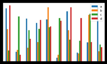
要生成堆积条形图,请pass stacked=True -
import pandas as pd
df = pd.DataFrame(np.random.rand(10,4),columns=['a','b','c','d')
df.plot.bar(stacked=True)
其output如下 -

要获得水平条形图,请使用barh方法 -
import pandas as pd
import numpy as np
df = pd.DataFrame(np.random.rand(10,4),columns=['a','b','c','d')
df.plot.barh(stacked=True)
其output如下 -

直方图(Histograms)
可以使用plot.hist()方法绘制直方图。 我们可以指定箱数。
import pandas as pd
import numpy as np
df = pd.DataFrame({'a':np.random.randn(1000)+1,'b':np.random.randn(1000),'c':
np.random.randn(1000) - 1}, columns=['a', 'b', 'c'])
df.plot.hist(bins=20)
其output如下 -
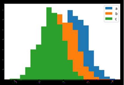
要为每列绘制不同的直方图,请使用以下代码 -
import pandas as pd
import numpy as np
df=pd.DataFrame({'a':np.random.randn(1000)+1,'b':np.random.randn(1000),'c':
np.random.randn(1000) - 1}, columns=['a', 'b', 'c'])
df.diff.hist(bins=20)
其output如下 -
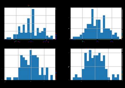
方块图
可以绘制Series.box.plot()调用Series.box.plot()和DataFrame.box.plot()或DataFrame.boxplot()来可视化每列中值的分布。
例如,这里是一个箱线图,表示在[0,1]上对均匀随机变量进行10次观测的五次试验。
import pandas as pd
import numpy as np
df = pd.DataFrame(np.random.rand(10, 5), columns=['A', 'B', 'C', 'D', 'E'])
df.plot.box()
其output如下 -

区域图
可以使用Series.plot.area()或DataFrame.plot.area()方法创建区域图。
import pandas as pd
import numpy as np
df = pd.DataFrame(np.random.rand(10, 4), columns=['a', 'b', 'c', 'd'])
df.plot.area()
其output如下 -

散点图
可以使用DataFrame.plot.scatter()方法创建散点图。
import pandas as pd
import numpy as np
df = pd.DataFrame(np.random.rand(50, 4), columns=['a', 'b', 'c', 'd'])
df.plot.scatter(x='a', y='b')
其output如下 -
饼形图
可以使用DataFrame.plot.pie()方法创建饼图。
import pandas as pd
import numpy as np
df = pd.DataFrame(3 * np.random.rand(4), index=['a', 'b', 'c', 'd'], columns=['x'])
df.plot.pie(subplots=True)
其output如下 -
Python Pandas - IO Tools
Pandas I/O API是一组顶级读取器函数,像pd.read_csv()一样访问,通常返回Pandas对象。
读取文本文件(或平面文件)的两个主要功能是read_csv()和read_table() 。 它们都使用相同的解析代码智能地将表格数据转换为DataFrame对象 -
pandas.read_csv(filepath_or_buffer, sep=',', delimiter=None, header='infer',
names=None, index_col=None, usecols=None
pandas.read_csv(filepath_or_buffer, sep='\t', delimiter=None, header='infer',
names=None, index_col=None, usecols=None
以下是csv文件数据的样子 -
S.No,Name,Age,City,Salary
1,Tom,28,Toronto,20000
2,Lee,32,HongKong,3000
3,Steven,43,Bay Area,8300
4,Ram,38,Hyderabad,3900
将此数据另存为temp.csv并对其执行操作。
S.No,Name,Age,City,Salary
1,Tom,28,Toronto,20000
2,Lee,32,HongKong,3000
3,Steven,43,Bay Area,8300
4,Ram,38,Hyderabad,3900
将此数据另存为temp.csv并对其执行操作。
read.csv
read.csv从csv文件中读取数据并创建DataFrame对象。
import pandas as pd
df=pd.read_csv("temp.csv")
print df
其output如下 -
S.No Name Age City Salary
0 1 Tom 28 Toronto 20000
1 2 Lee 32 HongKong 3000
2 3 Steven 43 Bay Area 8300
3 4 Ram 38 Hyderabad 3900
自定义索引
这指定csv文件中的列以使用index_col.自定义索引index_col.
import pandas as pd
df=pd.read_csv("temp.csv",index_col=['S.No'])
print df
其output如下 -
S.No Name Age City Salary
1 Tom 28 Toronto 20000
2 Lee 32 HongKong 3000
3 Steven 43 Bay Area 8300
4 Ram 38 Hyderabad 3900
转换器(Converters)
列的dtype可以作为dict传递。
import pandas as pd
df = pd.read_csv("temp.csv", dtype={'Salary': np.float64})
print df.dtypes
其output如下 -
S.No int64
Name object
Age int64
City object
Salary float64
dtype: object
默认情况下,Salary列的dtype是int ,但结果显示为float因为我们已经显式地转换了类型。
因此,数据看起来像浮动 -
S.No Name Age City Salary
0 1 Tom 28 Toronto 20000.0
1 2 Lee 32 HongKong 3000.0
2 3 Steven 43 Bay Area 8300.0
3 4 Ram 38 Hyderabad 3900.0
header_names
使用names参数指定标头的名称。
import pandas as pd
df=pd.read_csv("temp.csv", names=['a', 'b', 'c','d','e'])
print df
其output如下 -
a b c d e
0 S.No Name Age City Salary
1 1 Tom 28 Toronto 20000
2 2 Lee 32 HongKong 3000
3 3 Steven 43 Bay Area 8300
4 4 Ram 38 Hyderabad 3900
请注意,标题名称附加了自定义名称,但文件中的标题尚未消除。 现在,我们使用header参数删除它。
如果标题位于第一行之外的行中,则将行号传递给标题。 这将跳过前面的行。
import pandas as pd
df=pd.read_csv("temp.csv",names=['a','b','c','d','e'],header=0)
print df
其output如下 -
a b c d e
0 S.No Name Age City Salary
1 1 Tom 28 Toronto 20000
2 2 Lee 32 HongKong 3000
3 3 Steven 43 Bay Area 8300
4 4 Ram 38 Hyderabad 3900
skiprows
skiprows会跳过指定的行数。
import pandas as pd
df=pd.read_csv("temp.csv", skiprows=2)
print df
其output如下 -
2 Lee 32 HongKong 3000
0 3 Steven 43 Bay Area 8300
1 4 Ram 38 Hyderabad 3900
Python Pandas - Sparse Data
当任何匹配特定值的数据(NaN /缺失值,但可以选择任何值)被省略时,稀疏对象被“压缩”。 一个特殊的SparseIndex对象跟踪数据被“稀疏化”的位置。 这在一个例子中会更有意义。 所有标准的Pandas数据结构都应用to_sparse方法 -
import pandas as pd
import numpy as np
ts = pd.Series(np.random.randn(10))
ts[2:-2] = np.nan
sts = ts.to_sparse()
print sts
其output如下 -
0 -0.810497
1 -1.419954
2 NaN
3 NaN
4 NaN
5 NaN
6 NaN
7 NaN
8 0.439240
9 -1.095910
dtype: float64
BlockIndex
Block locations: array([0, 8], dtype=int32)
Block lengths: array([2, 2], dtype=int32)
出于内存效率的原因,存在稀疏对象。
现在让我们假设您有一个大的NA DataFrame并执行以下代码 -
import pandas as pd
import numpy as np
df = pd.DataFrame(np.random.randn(10000, 4))
df.ix[:9998] = np.nan
sdf = df.to_sparse()
print sdf.density
其output如下 -
0.0001
通过调用to_dense可以将任何稀疏对象转换回标准密集形式 -
import pandas as pd
import numpy as np
ts = pd.Series(np.random.randn(10))
ts[2:-2] = np.nan
sts = ts.to_sparse()
print sts.to_dense()
其output如下 -
0 -0.810497
1 -1.419954
2 NaN
3 NaN
4 NaN
5 NaN
6 NaN
7 NaN
8 0.439240
9 -1.095910
dtype: float64
稀疏Dtypes
稀疏数据应具有与其密集表示相同的dtype。 目前,支持float64, int64和booldtypes 。 根据原始dtype, fill_value default更改 -
float64 - np.nan
int64 - 0
bool - 错
让我们执行以下代码来理解相同的 -
import pandas as pd
import numpy as np
s = pd.Series([1, np.nan, np.nan])
print s
s.to_sparse()
print s
其output如下 -
0 1.0
1 NaN
2 NaN
dtype: float64
0 1.0
1 NaN
2 NaN
dtype: float64
Python Pandas - Caveats & Gotchas
警告意味着警告和陷阱意味着一个看不见的问题。
在Pandas中使用If/Truth语句
当您尝试将某些内容转换为bool时,Pandas会遵循提出错误的numpy惯例。 这种情况发生在if或者使用布尔运算时, or ,或者not 。 目前尚不清楚结果应该是什么。 它应该是真的,因为它不是zoleolength? 是的,因为有假值? 目前还不清楚,相反,熊猫提出了一个ValueError -
import pandas as pd
if pd.Series([False, True, False]):
print 'I am True'
其output如下 -
ValueError: The truth value of a Series is ambiguous. Use a.empty, a.bool() a.item(), a.any() or a.all().
if条件,不清楚如何处理它。 该错误暗示是否使用None或其中any of those 。
import pandas as pd
if pd.Series([False, True, False]).any():
print("I am any")
其output如下 -
I am any
要在布尔上下文中评估单元素pandas对象,请使用方法.bool() -
import pandas as pd
print pd.Series([True]).bool()
其output如下 -
True
按位布尔值
按位布尔运算符,如==和! =将返回一个布尔系列,这几乎总是需要的。
import pandas as pd
s = pd.Series(range(5))
print s==4
其output如下 -
0 False
1 False
2 False
3 False
4 True
dtype: bool
isin Operation
这将返回一个布尔系列,显示Series中的每个元素是否完全包含在传递的值序列中。
import pandas as pd
s = pd.Series(list('abc'))
s = s.isin(['a', 'c', 'e'])
print s
其output如下 -
0 True
1 False
2 True
dtype: bool
重新索引与ix Gotcha
许多用户会发现自己使用ix indexing capabilities作为从Pandas对象中选择数据的简洁方法 -
import pandas as pd
import numpy as np
df = pd.DataFrame(np.random.randn(6, 4), columns=['one', 'two', 'three',
'four'],index=list('abcdef'))
print df
print df.ix[['b', 'c', 'e']]
其output如下 -
one two three four
a -1.582025 1.335773 0.961417 -1.272084
b 1.461512 0.111372 -0.072225 0.553058
c -1.240671 0.762185 1.511936 -0.630920
d -2.380648 -0.029981 0.196489 0.531714
e 1.846746 0.148149 0.275398 -0.244559
f -1.842662 -0.933195 2.303949 0.677641
one two three four
b 1.461512 0.111372 -0.072225 0.553058
c -1.240671 0.762185 1.511936 -0.630920
e 1.846746 0.148149 0.275398 -0.244559
当然,在这种情况下,这与使用reindex方法reindex -
import pandas as pd
import numpy as np
df = pd.DataFrame(np.random.randn(6, 4), columns=['one', 'two', 'three',
'four'],index=list('abcdef'))
print df
print df.reindex(['b', 'c', 'e'])
其output如下 -
one two three four
a 1.639081 1.369838 0.261287 -1.662003
b -0.173359 0.242447 -0.494384 0.346882
c -0.106411 0.623568 0.282401 -0.916361
d -1.078791 -0.612607 -0.897289 -1.146893
e 0.465215 1.552873 -1.841959 0.329404
f 0.966022 -0.190077 1.324247 0.678064
one two three four
b -0.173359 0.242447 -0.494384 0.346882
c -0.106411 0.623568 0.282401 -0.916361
e 0.465215 1.552873 -1.841959 0.329404
有些人可能会得出结论,基于此, ix和reindex是100%等效的。 除了整数索引的情况之外,这是正确的。 例如,上述操作也可以表示为 -
import pandas as pd
import numpy as np
df = pd.DataFrame(np.random.randn(6, 4), columns=['one', 'two', 'three',
'four'],index=list('abcdef'))
print df
print df.ix[[1, 2, 4]]
print df.reindex([1, 2, 4])
其output如下 -
one two three four
a -1.015695 -0.553847 1.106235 -0.784460
b -0.527398 -0.518198 -0.710546 -0.512036
c -0.842803 -1.050374 0.787146 0.205147
d -1.238016 -0.749554 -0.547470 -0.029045
e -0.056788 1.063999 -0.767220 0.212476
f 1.139714 0.036159 0.201912 0.710119
one two three four
b -0.527398 -0.518198 -0.710546 -0.512036
c -0.842803 -1.050374 0.787146 0.205147
e -0.056788 1.063999 -0.767220 0.212476
one two three four
1 NaN NaN NaN NaN
2 NaN NaN NaN NaN
4 NaN NaN NaN NaN
重要的是要记住reindex is strict label indexing only 。 在索引包含整数和字符串的病态情况下,这可能会导致一些可能令人惊讶的结果。
Python Pandas - Comparison with SQL
由于许多潜在的Pandas用户对SQL有一定的了解,因此本页面旨在提供一些如何使用pandas执行各种SQL操作的示例。
import pandas as pd
url = 'https://raw.github.com/pandasdev/
pandas/master/pandas/tests/data/tips.csv'
tips=pd.read_csv(url)
print tips.head()
其output如下 -
total_bill tip sex smoker day time size
0 16.99 1.01 Female No Sun Dinner 2
1 10.34 1.66 Male No Sun Dinner 3
2 21.01 3.50 Male No Sun Dinner 3
3 23.68 3.31 Male No Sun Dinner 2
4 24.59 3.61 Female No Sun Dinner 4
SELECT
在SQL中,选择是使用您选择的以逗号分隔的列列表完成的(或*用于选择所有列) -
SELECT total_bill, tip, smoker, time
FROM tips
LIMIT 5;
使用Pandas,通过将列名列表传递给DataFrame来完成列选择 -
tips[['total_bill', 'tip', 'smoker', 'time']].head(5)
我们来检查完整的程序 -
import pandas as pd
url = 'https://raw.github.com/pandasdev/
pandas/master/pandas/tests/data/tips.csv'
tips=pd.read_csv(url)
print tips[['total_bill', 'tip', 'smoker', 'time']].head(5)
其output如下 -
total_bill tip smoker time
0 16.99 1.01 No Dinner
1 10.34 1.66 No Dinner
2 21.01 3.50 No Dinner
3 23.68 3.31 No Dinner
4 24.59 3.61 No Dinner
在没有列名列表的情况下调用DataFrame将显示所有列(类似于SQL的*)。
WHERE
SQL中的过滤是通过WHERE子句完成的。
SELECT * FROM tips WHERE time = 'Dinner' LIMIT 5;
DataFrame可以通过多种方式进行过滤; 最直观的是使用布尔索引。
tips[tips['time'] == 'Dinner'].head(5)
我们来检查完整的程序 -
import pandas as pd
url = 'https://raw.github.com/pandasdev/
pandas/master/pandas/tests/data/tips.csv'
tips=pd.read_csv(url)
print tips[tips['time'] == 'Dinner'].head(5)
其output如下 -
total_bill tip sex smoker day time size
0 16.99 1.01 Female No Sun Dinner 2
1 10.34 1.66 Male No Sun Dinner 3
2 21.01 3.50 Male No Sun Dinner 3
3 23.68 3.31 Male No Sun Dinner 2
4 24.59 3.61 Female No Sun Dinner 4
上面的语句将一系列True/False对象传递给DataFrame,返回所有行为True。
GroupBy
此操作获取整个数据集中每个组中的记录数。 例如,一个查询向我们提取性别留下的提示数量 -
SELECT sex, count(*)
FROM tips
GROUP BY sex;
熊猫的等价物是 -
tips.groupby('sex').size()
我们来检查完整的程序 -
import pandas as pd
url = 'https://raw.github.com/pandasdev/
pandas/master/pandas/tests/data/tips.csv'
tips=pd.read_csv(url)
print tips.groupby('sex').size()
其output如下 -
sex
Female 87
Male 157
dtype: int64
前N行
SQL使用LIMIT返回top n rows -
SELECT * FROM tips
LIMIT 5 ;
熊猫的等价物是 -
tips.head(5)
让我们看一下完整的例子 -
import pandas as pd
url = 'https://raw.github.com/pandas-dev/pandas/master/pandas/tests/data/tips.csv'
tips=pd.read_csv(url)
tips = tips[['smoker', 'day', 'time']].head(5)
print tips
其output如下 -
smoker day time
0 No Sun Dinner
1 No Sun Dinner
2 No Sun Dinner
3 No Sun Dinner
4 No Sun Dinner
这些是我们比较的几个基本操作,我们在Pandas Library的前几章中学到了这些操作。
