1. WIKI教程
2. Python深度学习
3. Implementations

Implementations

在深度学习的实施中，我们的目标是预测某个银行的客户流失或流失数据 - 客户可能会离开此银行服务。 使用的数据集相对较小，包含10000行，14列。 我们正在使用Anaconda发行版，以及Theano，TensorFlow和Keras等框架。 Keras建立在Tensorflow和Theano之上，后者作为其后端。

# Artificial Neural Network
# Installing Theano
pip install --upgrade theano
# Installing Tensorflow
pip install –upgrade tensorflow
# Installing Keras
pip install --upgrade keras

第1步:数据预处理

In[]:
# Importing the libraries
   import numpy as np
   import matplotlib.pyplot as plt
   import pandas as pd
# Importing the database
   dataset = pd.read_csv('Churn_Modelling.csv')

Step 2

我们创建数据集和目标变量的特征矩阵，即第14列，标记为“已退出”。

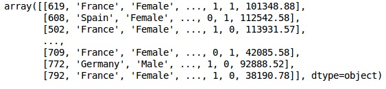
数据的初始外观如下所示 -

In[]:
X = dataset.iloc[:, 3:13].values
Y = dataset.iloc[:, 13].values
X

输出 (Output)

Step 3

Y

输出 (Output)

array([1, 0, 1, ..., 1, 1, 0], dtype = int64)

Step 4

我们通过编码字符串变量使分析更简单。 我们使用ScikitLearn函数'LabelEncoder'自动编码列中不同的标签，其值介于0到n_classes-1之间。

from sklearn.preprocessing import LabelEncoder, OneHotEncoder
labelencoder_X_1 = LabelEncoder() 
X[:,1] = labelencoder_X_1.fit_transform(X[:,1]) 
labelencoder_X_2 = LabelEncoder() 
X[:, 2] = labelencoder_X_2.fit_transform(X[:, 2])
X

输出 (Output)

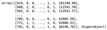
在上面的输出中，国家名称被替换为0,1和2; 男性和女性被0和1取代。

Step 5

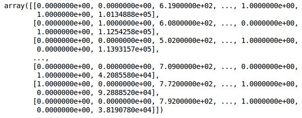
Labelling Encoded Data

我们使用相同的ScikitLearn库和另一个名为OneHotEncoder函数来传递创建虚拟变量的列号。

onehotencoder = OneHotEncoder(categorical features = [1])
X = onehotencoder.fit_transform(X).toarray()
X = X[:, 1:]
X

现在，前2列代表国家，第4列代表性别。

输出 (Output)

我们总是将数据划分为培训和测试部分; 我们在训练数据上训练我们的模型，然后检查模型在测试数据上的准确性，这有助于评估模型的效率。

Step 6

我们使用ScikitLearn的train_test_split函数将我们的数据分成训练集和测试集。 我们将列车 - 测试分流比保持在80:20。

#Splitting the dataset into the Training set and the Test Set
from sklearn.model_selection import train_test_split
X_train, X_test, y_train, y_test = train_test_split(X, y, test_size = 0.2)

一些变量的值为千，而一些变量的值为十或一。 我们扩展数据以使它们更具代表性。

Step 7

在此代码中，我们使用StandardScaler函数拟合和转换训练数据。 我们标准化我们的缩放比例，以便我们使用相同的拟合方法来转换/缩放测试数据。

# Feature Scaling

fromsklearn.preprocessing import StandardScaler 
sc = StandardScaler() 
X_train = sc.fit_transform(X_train) 
X_test = sc.transform(X_test)

输出 (Output)

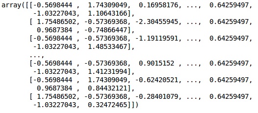
现在可以正确缩放数据。 最后，我们完成了数据预处理。 现在，我们将从我们的模型开始。

Step 8

我们在这里导入所需的模块。 我们需要Sequential模块来初始化神经网络，而密集模块则需要添加隐藏层。

# Importing the Keras libraries and packages 
import keras 
from keras.models import Sequential 
from keras.layers import Dense

Step 9

我们将该模型命名为Classifier，因为我们的目标是对客户流失进行分类。 然后我们使用Sequential模块进行初始化。

#Initializing Neural Network 
classifier = Sequential()

第10步

我们使用密集函数逐个添加隐藏层。 在下面的代码中，我们将看到许多参数。

我们的第一个参数是output_dim 。 它是我们添加到该层的节点数。 init是Stochastic Gradient Decent的初始化。 在神经网络中，我们为每个节点分配权重。 在初始化时，权重应接近零，我们使用统一函数随机初始化权重。 input_dim参数仅适用于第一层，因为模型不知道输入变量的数量。 这里输入变量的总数是11.在第二层中，模型自动知道来自第一个隐藏层的输入变量的数量。

执行以下代码行来添加输入图层和第一个隐藏图层 -

classifier.add(Dense(units = 6, kernel_initializer = 'uniform', 
activation = 'relu', input_dim = 11))

执行以下代码行添加第二个隐藏层 -

classifier.add(Dense(units = 6, kernel_initializer = 'uniform', 
activation = 'relu'))

执行以下代码行来添加输出层 -

classifier.add(Dense(units = 1, kernel_initializer = 'uniform', 
activation = 'sigmoid'))

第11步

Compiling the ANN

到目前为止，我们已经为分类器添加了多个图层。 我们现在将使用compile方法编译它们。 在最终编译控件中添加的参数完成了神经网络。因此，我们需要在此步骤中小心。

以下是对这些论点的简要解释。

第一个参数是Optimizer 。这是一个用于查找最佳权重集的算法。 该算法称为Stochastic Gradient Descent (SGD) 。 在这里，我们使用了几种类型中的一种，称为“亚当优化器”。 新元取决于损失，因此我们的第二个参数是损失。 如果我们的因变量是二进制的，我们使用称为'binary_crossentropy'对数损失函数，如果我们的因变量在输出中有两个以上的类别，那么我们使用'categorical_crossentropy' 。 我们希望基于accuracy来提高神经网络的性能，因此我们将metrics添加为准确性。

# Compiling Neural Network 
classifier.compile(optimizer = 'adam', loss = 'binary_crossentropy', metrics = ['accuracy'])

第12步

在此步骤中需要执行许多代码。

将ANN安装到训练集

我们现在在训练数据上训练我们的模型。 我们使用fit方法来拟合我们的模型。 我们还优化了重量以提高模型效率。 为此，我们必须更新权重。 Batch size是我们更新权重之后的观察数量。 Epoch是迭代的总数。 批量大小和时期的值通过试错法选择。

classifier.fit(X_train, y_train, batch_size = 10, epochs = 50)

进行预测并评估模型

# Predicting the Test set results
y_pred = classifier.predict(X_test)
y_pred = (y_pred > 0.5)

预测一个新的观察

# Predicting a single new observation
"""Our goal is to predict if the customer with the following data will leave the bank:
Geography: Spain
Credit Score: 500
Gender: Female
Age: 40
Tenure: 3
Balance: 50000
Number of Products: 2
Has Credit Card: Yes
Is Active Member: Yes

第13步

Predicting the test set result

预测结果将为您提供客户离开公司的概率。 我们将该概率转换为二进制0和1。

# Predicting the Test set results 
y_pred = classifier.predict(X_test) 
y_pred = (y_pred > 0.5)

new_prediction = classifier.predict(sc.transform
(np.array([[0.0, 0, 500, 1, 40, 3, 50000, 2, 1, 1, 40000]])))
new_prediction = (new_prediction > 0.5)

第14步

这是我们评估模型性能的最后一步。 我们已经有了原始结果，因此我们可以构建混淆矩阵来检查模型的准确性。

Making the Confusion Matrix

from sklearn.metrics import confusion_matrix
cm = confusion_matrix(y_test, y_pred)
print (cm)

输出 (Output)

loss: 0.3384 acc: 0.8605
[ [1541 54]
[230 175] ]

从混淆矩阵中，我们模型的精度可以计算为 -

Accuracy = 1541+175/2000=0.858

We achieved 85.8% accuracy ，这很好。

前向传播算法

在本节中，我们将学习如何编写代码来进行简单神经网络的前向传播（预测） -

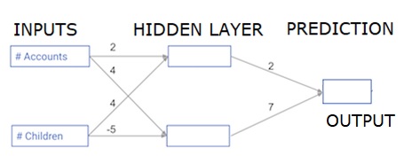
每个数据点都是客户。 第一个输入是他们有多少个帐户，第二个输入是他们有多少个孩子。 该模型将预测用户在明年进行的交易数量。

输入数据被预加载为输入数据，并且权重在称为权重的字典中。 隐藏层中第一个节点的权重数组为权重['node_0']，隐藏层中第二个节点的权重数据分别为权重['node_1']。

馈入输出节点的权重可用于权重。

整流线性激活函数

“激活功能”是在每个节点上工作的功能。 它将节点的输入转换为某个输出。

经过整流的线性激活功能（称为ReLU ）广泛用于非常高性能的网络中。 此函数将单个数字作为输入，如果输入为负，则返回0;如果输入为正，则输入为输出。

以下是一些例子 -

• relu（4）= 4
• relu（-2）= 0

我们填写relu（）函数的定义 -

• 我们使用max（）函数计算relu（）输出的值。
• 我们将relu（）函数应用于node_0_input以计算node_0_output。
• 我们将relu（）函数应用于node_1_input以计算node_1_output。

import numpy as np
input_data = np.array([-1, 2])
weights = {
   'node_0': np.array([3, 3]),
   'node_1': np.array([1, 5]),
   'output': np.array([2, -1])
}
node_0_input = (input_data * weights['node_0']).sum()
node_0_output = np.tanh(node_0_input)
node_1_input = (input_data * weights['node_1']).sum()
node_1_output = np.tanh(node_1_input)
hidden_layer_output = np.array(node_0_output, node_1_output)
output =(hidden_layer_output * weights['output']).sum()
print(output)
def relu(input):
   '''Define your relu activation function here'''
   # Calculate the value for the output of the relu function: output
   output = max(input,0)
      # Return the value just calculated
   return(output)
# Calculate node 0 value: node_0_output
node_0_input = (input_data * weights['node_0']).sum()
node_0_output = relu(node_0_input)
# Calculate node 1 value: node_1_output
node_1_input = (input_data * weights['node_1']).sum()
node_1_output = relu(node_1_input)
# Put node values into array: hidden_layer_outputs
hidden_layer_outputs = np.array([node_0_output, node_1_output])
# Calculate model output (do not apply relu)
odel_output = (hidden_layer_outputs * weights['output']).sum()
print(model_output)# Print model output

输出 (Output)

0.9950547536867305
-3

将网络应用于许多观察/行数据

在本节中，我们将学习如何定义名为predict_with_network（）的函数。 此函数将生成多个数据观测的预测，从上面的网络中获取input_data。 正在使用上述网络中给出的权重。 还使用了relu（）函数定义。

让我们定义一个名为predict_with_network（）的函数，它接受两个参数 - input_data_row和weights - 并从网络返回一个预测作为输出。

我们计算每个节点的输入和输出值，将它们存储为:node_0_input，node_0_output，node_1_input和node_1_output。

要计算节点的输入值，我们将相关数组相乘并计算它们的总和。

要计算节点的输出值，我们将relu（）函数应用于节点的输入值。 我们使用'for循环'来迭代input_data -

我们还使用predict_with_network（）为input_data的每一行生成预测 - input_data_row。 我们还将每个预测附加到结果中。

# Define predict_with_network()
def predict_with_network(input_data_row, weights):
   # Calculate node 0 value
   node_0_input = (input_data_row * weights['node_0']).sum()
   node_0_output = relu(node_0_input)
   # Calculate node 1 value
   node_1_input = (input_data_row * weights['node_1']).sum()
   node_1_output = relu(node_1_input)
   # Put node values into array: hidden_layer_outputs
   hidden_layer_outputs = np.array([node_0_output, node_1_output])
   # Calculate model output
   input_to_final_layer = (hidden_layer_outputs*weights['output']).sum()
   model_output = relu(input_to_final_layer)
# Return model output
   return(model_output)
# Create empty list to store prediction results
results = []
for input_data_row in input_data:
   # Append prediction to results
   results.append(predict_with_network(input_data_row, weights))
print(results)# Print results

输出 (Output)

[0, 12]

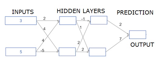
深层多层神经网络

在这里，我们编写代码来为具有两个隐藏层的神经网络进行前向传播。 每个隐藏层都有两个节点。 输入数据已预先加载为input_data 。 第一个隐藏层中的节点称为node_0_0和node_0_1。

它们的权重分别作为权重['node_0_0']和权重['node_0_1']预先加载。

第二个隐藏层中的节点称为node_1_0 and node_1_1 。 它们的权重分别作为weights['node_1_0']和weights['node_1_1']预先加载。

然后，我们使用预加载为weights['output']从隐藏节点创建模型输出。

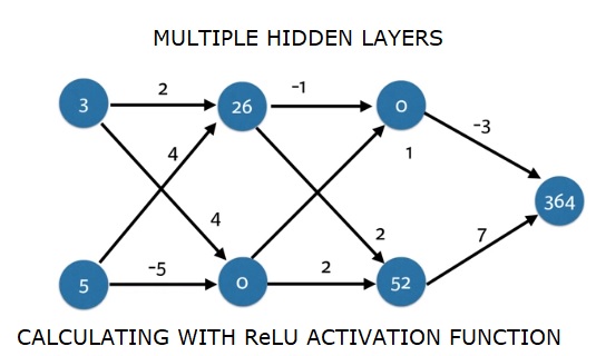
我们使用权重权重['node_0_0']和给定的input_data来计算node_0_0_input。 然后应用relu（）函数获取node_0_0_output。

我们对node_0_1_input执行与上面相同的操作以获取node_0_1_output。

我们使用权重权重['node_1_0']和第一个隐藏层的输出 - hidden_​​0_outputs来计算node_1_0_input。 然后我们应用relu（）函数来获取node_1_0_output。

我们对node_1_1_input执行与上述相同的操作以获取node_1_1_output。

我们使用权重['output']和第二个隐藏层hidden_​​1_outputs数组的输出计算model_output。 我们不将relu（）函数应用于此输出。

import numpy as np
input_data = np.array([3, 5])
weights = {
   'node_0_0': np.array([2, 4]),
   'node_0_1': np.array([4, -5]),
   'node_1_0': np.array([-1, 1]),
   'node_1_1': np.array([2, 2]),
   'output': np.array([2, 7])
}
def predict_with_network(input_data):
   # Calculate node 0 in the first hidden layer
   node_0_0_input = (input_data * weights['node_0_0']).sum()
   node_0_0_output = relu(node_0_0_input)
   # Calculate node 1 in the first hidden layer
   node_0_1_input = (input_data*weights['node_0_1']).sum()
   node_0_1_output = relu(node_0_1_input)
   # Put node values into array: hidden_0_outputs
   hidden_0_outputs = np.array([node_0_0_output, node_0_1_output])
   # Calculate node 0 in the second hidden layer
   node_1_0_input = (hidden_0_outputs*weights['node_1_0']).sum()
   node_1_0_output = relu(node_1_0_input)
   # Calculate node 1 in the second hidden layer
   node_1_1_input = (hidden_0_outputs*weights['node_1_1']).sum()
   node_1_1_output = relu(node_1_1_input)
   # Put node values into array: hidden_1_outputs
   hidden_1_outputs = np.array([node_1_0_output, node_1_1_output])
   # Calculate model output: model_output
   model_output = (hidden_1_outputs*weights['output']).sum()
      # Return model_output
   return(model_output)
output = predict_with_network(input_data)
print(output)

输出 (Output)

364